Machine learning for drug sensitivity prediction (Part 1): using autoencoders to extract deep features from DepMap OMICS
R
DepMap
Autoencoder
Multi-omics
Machine Learning
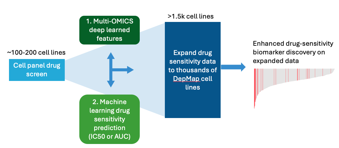
During my time in the industry, I have analyzed quite a few cell panel screens aiming to identify biomarkers of drug sensitivity. These screens are often carried out by CROs, and due to the costs associated with these experiments, the number of cell lines screened is often limited. Very often the average number of cell lines in each lineage is less than 10, which limits the power of biomarker detection. One way to mitigate this issue is to train a machine learning model based on the available cell lines and their corresponding DepMap omics data, and then use the trained model to predict sensitivity across thousands of DepMap cell lines. This expanded set of predicted sensitivities can then be used for biomarker detection with improved power.
In this post, I want to explore whether using autoencoders (AE) to compress high-dimensional omics data into deep features can improve drug sensitivity prediction accuracy. The concept can be summarized in the figure below:
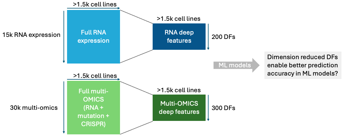
I demonstrate how to use AE to compress DepMap RNA expression data alone and multi-omics data (RNA expression + mutation + CRISPR dependency scores) into deep features. I then visualize and compare the embeddings from RNA alone vs. multi-omics data. In future work (part 2), I will compare the drug sensitivity prediction accuracy using deep features vs. full omics data.
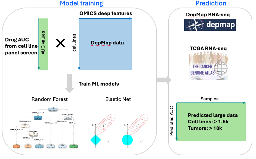
These concepts can be summarized in Component 1 (AE embedding) and 2 (ML training) in the following figures:
Component 1: Autoencoder embedding
Component 2: ML training and prediction
Introduction
Background: Cell panel drug screens are very useful during drug development in identifying sensitive biomarkers and understanding the mechanism-of-action; however, it can be costly and often result in only up to hundreds of cell lines available, limiting the power of biomarker detection. By leveraging machine learning (ML) approaches, one can expand sensitivity prediction to thousands of DepMap cell lines and thus improve the power of biomarker detection.
Problem: DepMap OMICS data are high-dimensional, and such high-dimensional data may hinder ML prediction due to overfitting problems and noisy data.
Proposal: By leveraging AutoEncoder (AE), a deep learning approach, high-dimensional OMICS data can be compressed into Deep Features (DF), thus overcoming the problem of overfitting and resulting in better drug sensitivity prediction accuracy. Unlike traditional dimensionality reduction methods (e.g., PCA), AE can capture non-linear relationships in the data, leading to more informative embeddings.
Setup and Libraries
library(tidyverse)
library(data.table)
library(ggpubr)
library(h2o)
library(umap)
library(ggrepel)
library(microViz)
Aim 1: RNA Expression Autoencoder
First, we use an autoencoder to embed cell lines based on RNA expression data alone.
Data Loading and Preprocessing
We filter for high-variance genes to reduce noise and dimensionality before feeding the data into the autoencoder.
# load data: RNA expression
# Note: these RData files contain preprocessed data matrices with matched sample information
# DepMap data can be downloaded from https://depmap.org/portal/download/
# Here I am using the 24Q2 release
load("CCLE_24Q2_GE_match_sample_info.RData") # rows are cell lines, columns are genes, values are RNA-seq log2(TPM+1)
load("sample_info_match_biomarkers.RData") # sample info with lineage annotations

# remove low variance genes
ge_var <- apply(ccle_ge_match_sam, 2, var, na.rm = TRUE)
ge_dat_hv <- ccle_ge_match_sam[, which(ge_var > quantile(ge_var, 0.2))] # select high variance genes (top 80th percentile)

# remove any cell lines (rows) that contains NAs
ge_dat_hv <- ge_dat_hv |> na.omit()

# standardize the data
ge_dat_hv <- scale(ge_dat_hv) |> as.data.frame()
Let’s see what the RNA expression data looks like:
ge_dat_hv[1:5, 1:5] |>
    rownames_to_column("CellLine") |>
gt::gt(rowname_col = "CellLine")| TSPAN6 | DPM1 | FIRRM | FGR | CFH | |
|---|---|---|---|---|---|
| NIHOVCAR3 | 1.0926276 | 1.5011722 | 0.6858109 | -0.3170060 | -0.5737765 |
| HL60 | -1.9693314 | -1.2610758 | -0.6848542 | 3.0178580 | -0.8997009 |
| CACO2 | 1.1699782 | 2.0373191 | 0.2826820 | -0.3517010 | -0.9468198 |
| HEL | -0.7463001 | -1.6419864 | 0.3162823 | 0.3703802 | 1.2136680 |
| HEL9217 | -0.5779999 | -0.9799468 | 2.0368574 | -0.1876538 | 1.5663762 |
Let’s see what the sample info looks like:
sample_info[1:5, ] |> gt::gt()| ModelID | StrippedCellLineName | CCLEName | OncotreeLineage | OncotreeSubtype | OncotreePrimaryDisease | LegacySubSubtype | LegacyMolecularSubtype | PatientMolecularSubtype |
|---|---|---|---|---|---|---|---|---|
| ACH-000001 | NIHOVCAR3 | NIHOVCAR3_OVARY | Ovary/Fallopian Tube | High-Grade Serous Ovarian Cancer | Ovarian Epithelial Tumor | high_grade_serous | ||
| ACH-000002 | HL60 | HL60_HAEMATOPOIETIC_AND_LYMPHOID_TISSUE | Myeloid | Acute Myeloid Leukemia | Acute Myeloid Leukemia | M3 | TP53(del), CDKN2A and NRAS mutations [PubMed=288488], No PML-RARA fusion | |
| ACH-000003 | CACO2 | CACO2_LARGE_INTESTINE | Bowel | Colon Adenocarcinoma | Colorectal Adenocarcinoma | |||
| ACH-000004 | HEL | HEL_HAEMATOPOIETIC_AND_LYMPHOID_TISSUE | Myeloid | Acute Myeloid Leukemia | Acute Myeloid Leukemia | M6 | JAK2 and TP53 mutations, | |
| ACH-000005 | HEL9217 | HEL9217_HAEMATOPOIETIC_AND_LYMPHOID_TISSUE | Myeloid | Acute Myeloid Leukemia | Acute Myeloid Leukemia | M6 | JAK2 and TP53 mutations |
Model Training
We perform a hyperparameter grid search to find the optimal autoencoder architecture.
# Hyperparameter search grid to find best AE model
h2o.init(nthreads = 20, max_mem_size = "60G") # initialize H2O with 20 threads and 60GB memory
rna_h2o <- as.h2o(ge_dat_hv)

hyper_grid <- list(hidden = list(
    c(1000, 500, 1000),
    c(1000, 500, 200, 500, 1000),
    c(1000, 100, 50, 100, 1000),
    c(1000, 500, 100, 500, 1000),
    c(2000, 1000, 200, 1000, 2000),
    c(1000, 500, 300, 500, 1000)
))

ae_grid <- h2o.grid(
    algorithm = "deeplearning",
    x = colnames(rna_h2o),
    training_frame = rna_h2o,
    grid_id = "RNA_ae1",
    autoencoder = TRUE,
    activation = "TanhWithDropout", # I've also tried "RectifierWithDropout" but seemed to encounter exploding gradients
    hyper_params = hyper_grid,
    nesterov_accelerated_gradient = TRUE,
    epochs = 30,
    stopping_rounds = 5,
    seed = 524
)

# get grid results, sorted by reconstruction error (MSE)
h2o.getGrid("RNA_ae1", sort_by = "mse", decreasing = FALSE)

# AE learning with best parameters (selected from grid search)
ae_model <- h2o.deeplearning(
    x = colnames(rna_h2o),
    training_frame = rna_h2o,
    autoencoder = TRUE,
    hidden = c(1000, 500, 200, 500, 1000),
    hidden_dropout_ratios = c(0.5, 0.5, 0.5, 0.5, 0.5),
    activation = "TanhWithDropout",
    epochs = 30,
    stopping_rounds = 5,
    nesterov_accelerated_gradient = TRUE,
    seed = 524
)

# extract the compressed features
compressed_features <- h2o.deepfeatures(ae_model, rna_h2o, layer = 3) |> as.data.frame() # get deep features from the middle layer
rownames(compressed_features) <- rownames(ge_dat_hv)

# Save results
fwrite(compressed_features, file = "./results/output_files/RNA_AE_compressed_features.csv", sep = ",", row.names = TRUE)
h2o.shutdown()
I want to point out that the choice of architecture (number of layers and nodes) and hyperparameters (dropout rates, activation functions) can significantly impact the quality of the learned embeddings. For example, using batch normalization layers or experimenting with different activation functions (e.g., ReLU, Leaky ReLU) might yield better results depending on the data characteristics. Readers interested in this topic should explore more sophisticated MLP training platform like Keras and TensorFlow.
Aim 2: Multi-omics Autoencoder
Next, we integrate RNA expression, mutation data (damaging, hotspot), and CRISPR dependency scores.
Data Integration
We process each data type separately (filtering, standardizing) and then combine them into a single multi-omics dataset.
# load data (all rows are cell lines and columns are genes)
load("CCLE_24Q2_GE_match_sample_info.RData") # RNA expression
load("DepMap_24Q2_Chronos_match_sample_info.RData") # CRISPR dependency scores (Chronos)
load("CCLE_24Q2_DAMMUT_match_sample_info.RData") # Damaging mutations (0: non-mutated, 1: mutated heterozygous, 2: mutated homozygous)
load("CCLE_24Q2_HOTMUT_match_sample_info.RData") # Hotspot mutations (0: non-mutated, 1: mutated heterozygous, 2: mutated homozygous)
load("sample_info_match_biomarkers.RData") # sample info

# RNA processing
ge_var <- apply(ccle_ge_match_sam, 2, var, na.rm = TRUE)
ge_dat_hv <- ccle_ge_match_sam[, which(ge_var > quantile(ge_var, 0.2))]
ge_dat_hv <- scale(ge_dat_hv) |> as.data.frame()

# Mutation processing
dam_mut_dat_filt <- dammut_dat_match_sam[, which(apply(na.omit(dammut_dat_match_sam), 2, function(x) sum(x != 0)) > 20)] # filter genes with >20 mutated events across cell lines
hot_mut_dat_filt <- hotmut_dat_match_sam[, which(apply(na.omit(hotmut_dat_match_sam), 2, function(x) sum(x != 0)) > 20)]

# CRISPR processing
crispr_var <- apply(chronos_dat_match_sam, 2, var, na.rm = TRUE)
crispr_dat_hv <- chronos_dat_match_sam[, which(crispr_var > quantile(crispr_var, 0.2))]
crispr_dat_hv <- scale(crispr_dat_hv) |> as.data.frame()

# Combine data
colnames(ge_dat_hv) <- paste0(colnames(ge_dat_hv), "_RNA")
colnames(dam_mut_dat_filt) <- paste0(colnames(dam_mut_dat_filt), "_DAMMUT")
colnames(hot_mut_dat_filt) <- paste0(colnames(hot_mut_dat_filt), "_HOTMUT")
colnames(crispr_dat_hv) <- paste0(colnames(crispr_dat_hv), "_CRISPR")

multi_omics_dat <- cbind(ge_dat_hv, dam_mut_dat_filt, hot_mut_dat_filt, crispr_dat_hv)

# Remove rows with too many NAs
multi_omics_dat <- multi_omics_dat[rowSums(is.na(multi_omics_dat)) <= ncol(multi_omics_dat) * 0.8, ] # keep rows with <=80% NAs
Multi-omics Model Training
We train another autoencoder on this combined dataset.
h2o.init(nthreads = 20, max_mem_size = "60G")
rna_h2o <- as.h2o(multi_omics_dat)

# (Grid search code omitted for brevity, similar to Aim 1)

# AE learning with best parameters
ae_model <- h2o.deeplearning(
    x = colnames(rna_h2o),
    training_frame = rna_h2o,
    autoencoder = TRUE,
    hidden = c(1000, 500, 300, 500, 1000),
    hidden_dropout_ratios = c(0.5, 0.5, 0.5, 0.5, 0.5),
    activation = "TanhWithDropout",
    epochs = 30,
    stopping_rounds = 5,
    nesterov_accelerated_gradient = TRUE,
    seed = 524
)

compressed_features <- h2o.deepfeatures(ae_model, rna_h2o, layer = 3) |> as.data.frame() # here we take 300-dim deep features
rownames(compressed_features) <- rownames(multi_omics_dat)

fwrite(compressed_features, file = "./results/output_files/MultiOmics_AE_compressed_features.csv", sep = ",", row.names = TRUE)
h2o.shutdown()
Aim 3: Visualization and Comparison
Finally, we visualize the embeddings using UMAP and compare the clustering with known lineages.
Here we are testing if the deep features preserve and/or enrich biological signals present in the original data.
Full RNA UMAP (without Autoencoder)
# load data
load("CCLE_24Q2_GE_match_sample_info.RData")
load("sample_info_match_biomarkers.RData")

# remove low variance genes
ge_var <- apply(ccle_ge_match_sam, 2, var, na.rm = TRUE) # calculate variance for each gene
sum(ge_var > quantile(ge_var, 0.2)) # how many genes passed variance cutoff: 15322
ge_dat_hv <- ccle_ge_match_sam[, which(ge_var > quantile(ge_var, 0.2))] # select high variance genes

# standardize the data and match with sample info
ge_dat_hv <- scale(ge_dat_hv) |>
    as.data.frame() |>
    na.omit()
sample_info <- sample_info[match(rownames(ge_dat_hv), sample_info$StrippedCellLineName), ]
all(rownames(ge_dat_hv) == sample_info$StrippedCellLineName)

# Run UMAP
library(umap)
umap_dat <- umap(
    ge_dat_hv,
    n_components = 2,
    n_neighbors = 50,
    random_state = 524,
    verbose = TRUE,
    n_threads = 15
)
umap_dat <- as.data.frame(umap_dat$layout)
umap_dat$cell_line <- sample_info$StrippedCellLineName
umap_dat$lineage <- sample_info$OncotreeLineage
umap_dat$subtype <- sample_info$OncotreeSubtype

# Plot UMAP embedding colored by lineage
ggplot(umap_dat, aes(V1, -V2, color = lineage, fill = lineage)) +
    geom_point(size = 3, alpha = 0.5) +
    scale_fill_manual(values = distinct_palette(n = length(unique(umap_dat$lineage)), pal = "brewerPlus", add = "lightgrey")) +
    scale_color_manual(values = distinct_palette(n = length(unique(umap_dat$lineage)), pal = "brewerPlus", add = "lightgrey")) +
    theme_classic(base_size = 20) +
    # add lineage labels at the center of each lineage cluster
    geom_label_repel(
        data = umap_dat %>%
            group_by(lineage) %>%
            summarize(V1 = median(V1), V2 = median(V2)),
        aes(label = lineage, color = lineage),
        size = 4,
        # color = "black",
        fill = "white",
        alpha = 0.7,
        show.legend = FALSE,
        max.overlaps = 100
    ) +
    theme(
        legend.position = "none",
        legend.title = element_text(size = 10),
        legend.text = element_text(size = 10)
    ) +
    labs(
        x = "UMAP1",
        y = "UMAP2",
        title = "UMAP of full CCLE RNA expression (no AE)"
    )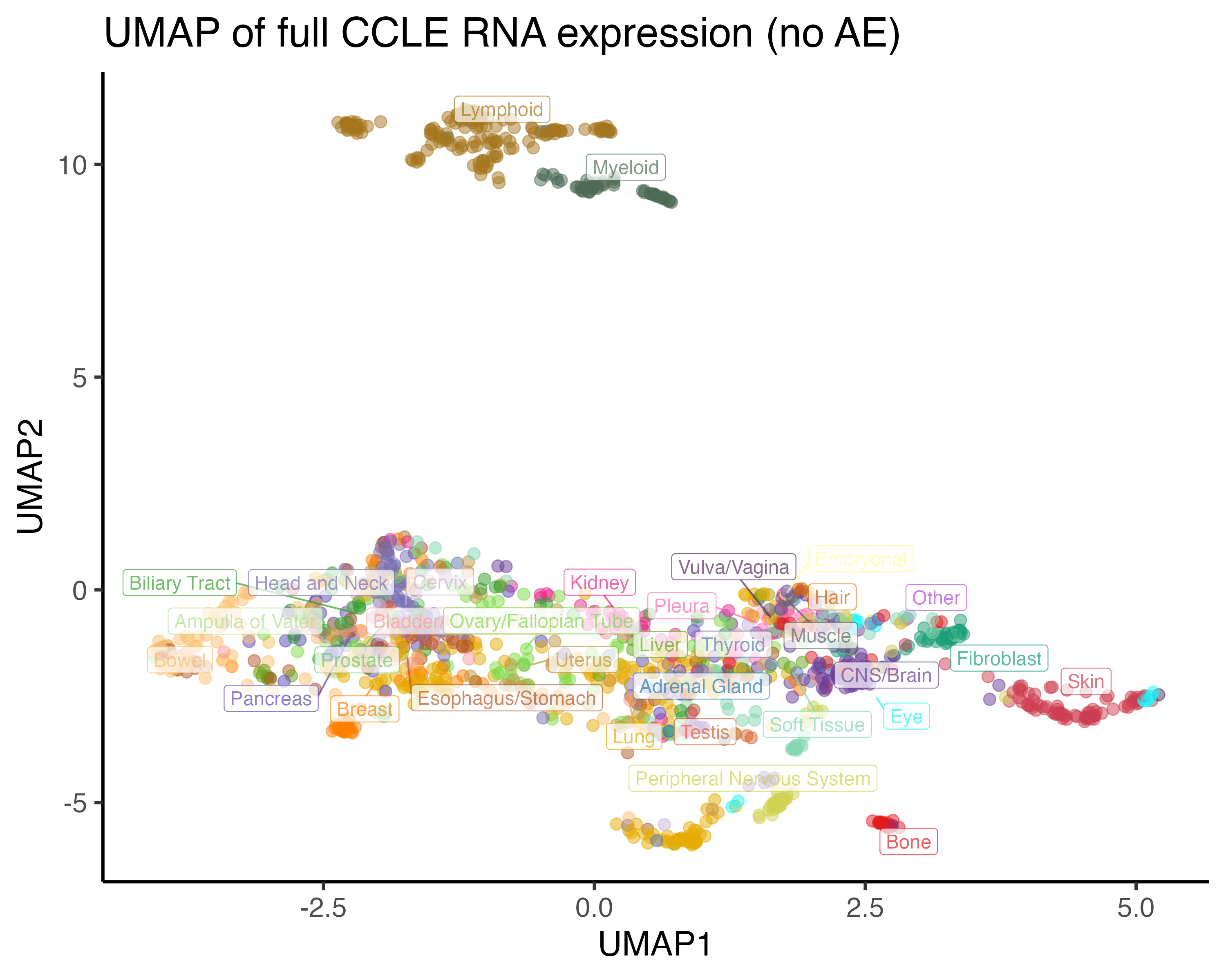
As you can see, the full RNA data UMAP already shows some clustering by lineage, indicating that the transcriptomic profiles capture biological differences among cell lines.
RNA deep features UMAP
# Load compressed features
RNA_AE_compressed_features <- fread("./results/output_files/RNA_AE_compressed_features.csv", data.table = FALSE) |>
    column_to_rownames(var = "V1")
RNA_AE_compressed_features <- RNA_AE_compressed_features[rowSums(RNA_AE_compressed_features) != 0, ]

# Match with sample info
sample_info <- sample_info[match(rownames(RNA_AE_compressed_features), sample_info$StrippedCellLineName), ]

# Run UMAP
umap_dat <- umap(RNA_AE_compressed_features, n_components = 2, n_neighbors = 50, random_state = 524)
umap_dat <- as.data.frame(umap_dat$layout)
umap_dat$lineage <- sample_info$OncotreeLineage

# Plot
ggplot(umap_dat, aes(V1, V2, color = lineage, fill = lineage)) +
    geom_point(size = 3, alpha = 0.5) +
    scale_fill_manual(values = distinct_palette(n = length(unique(umap_dat$lineage)), pal = "brewerPlus", add = "lightgrey")) +
    scale_color_manual(values = distinct_palette(n = length(unique(umap_dat$lineage)), pal = "brewerPlus", add = "lightgrey")) +
    theme_classic(base_size = 20) +
    geom_label_repel(
        data = umap_dat %>% group_by(lineage) %>% summarize(V1 = median(V1), V2 = median(V2)),
        aes(label = lineage, color = lineage),
        size = 4, fill = "white", alpha = 0.7, show.legend = FALSE, max.overlaps = 100
    ) +
    theme(legend.position = "none") +
    labs(title = "UMAP of AE compressed CCLE RNA expression")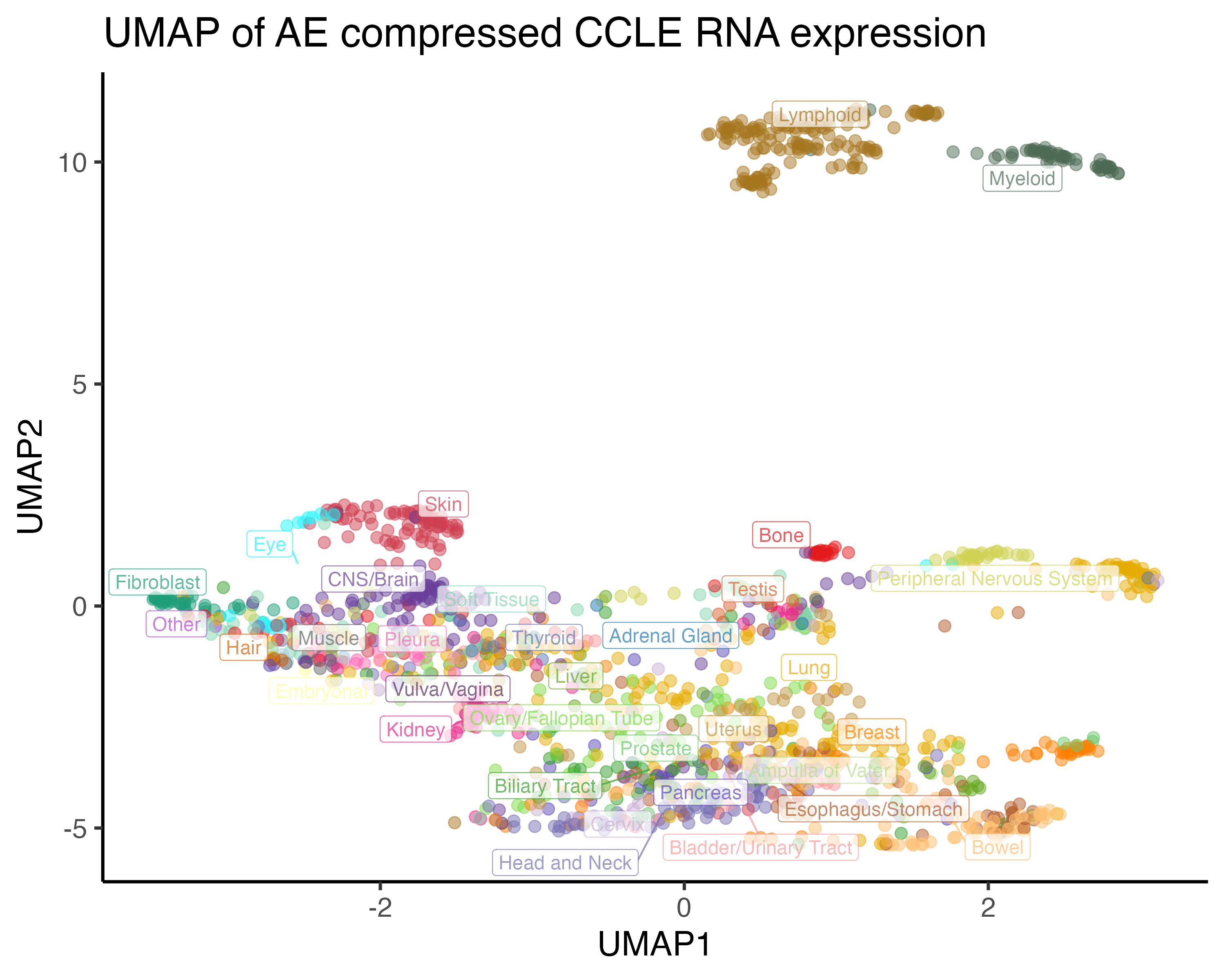
The RNA deep features UMAP also shows clustering by lineage, similar to the full RNA data, indicating that the autoencoder effectively preserves the biological signal in a lower-dimensional space.
Multi-omics deep features UMAP
# Load compressed features
MultiOmics_AE_compressed_features <- fread("./results/output_files/MultiOmics_AE_compressed_features.csv", data.table = FALSE) |>
    column_to_rownames(var = "V1")
MultiOmics_AE_compressed_features <- MultiOmics_AE_compressed_features[rowSums(MultiOmics_AE_compressed_features) != 0, ]

# Match with sample info
sample_info <- sample_info[match(rownames(MultiOmics_AE_compressed_features), sample_info$StrippedCellLineName), ]

# Run UMAP
umap_dat <- umap(MultiOmics_AE_compressed_features, n_components = 2, n_neighbors = 50, random_state = 524)
umap_dat <- as.data.frame(umap_dat$layout)
umap_dat$lineage <- sample_info$OncotreeLineage

# Plot
ggplot(umap_dat, aes(-V1, -V2, color = lineage, fill = lineage)) +
    geom_point(size = 3, alpha = 0.5) +
    scale_fill_manual(values = distinct_palette(n = length(unique(umap_dat$lineage)), pal = "brewerPlus", add = "lightgrey")) +
    scale_color_manual(values = distinct_palette(n = length(unique(umap_dat$lineage)), pal = "brewerPlus", add = "lightgrey")) +
    theme_classic(base_size = 20) +
    geom_label_repel(
        data = umap_dat %>% group_by(lineage) %>% summarize(V1 = median(V1), V2 = median(V2)),
        aes(label = lineage, color = lineage),
        size = 4, fill = "white", alpha = 0.7, show.legend = FALSE, max.overlaps = 100
    ) +
    theme(legend.position = "none") +
    labs(title = "UMAP of AE compressed CCLE Multi-omics")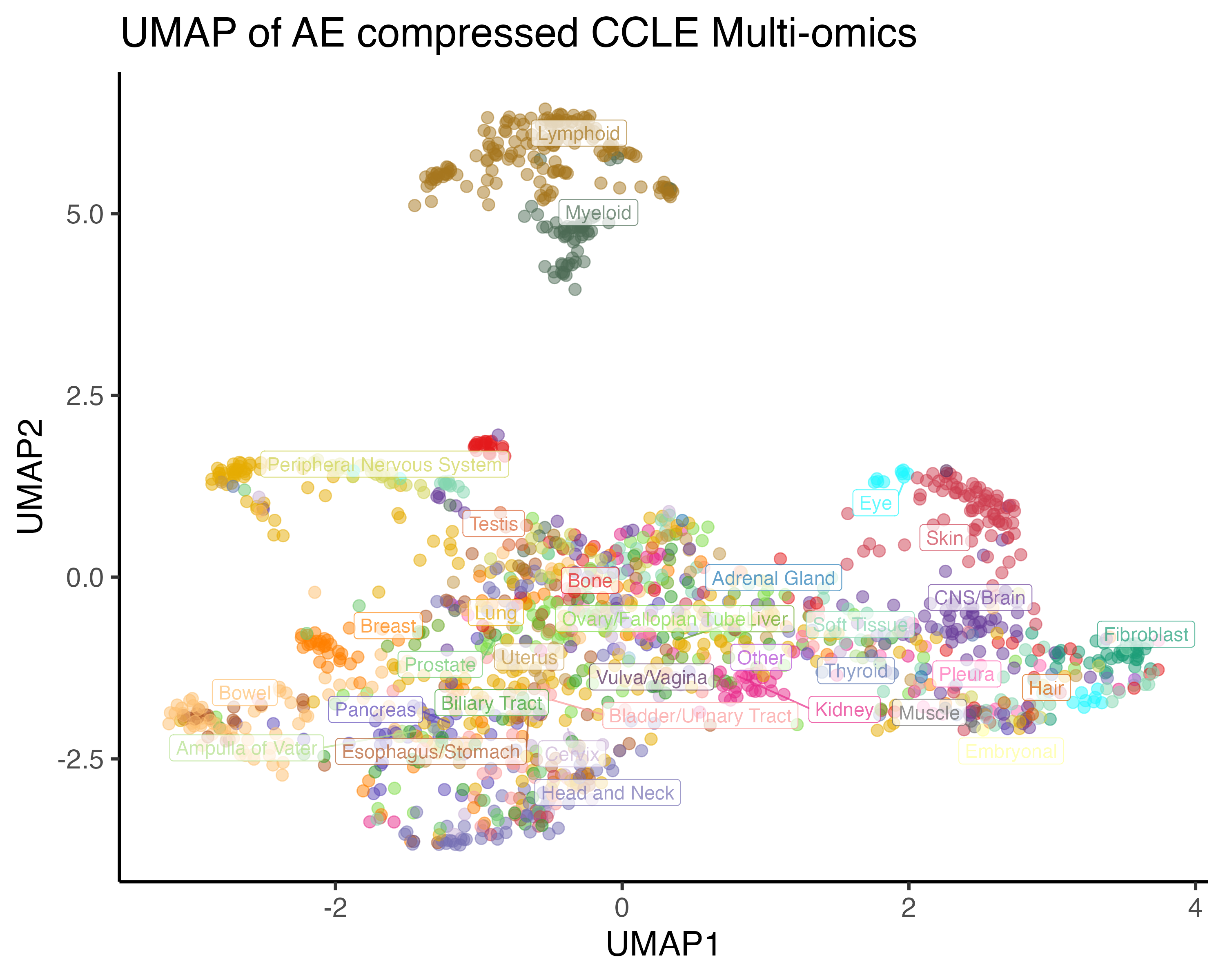
The AE embedded multi-OMICS appears to increase the granularity of cell line clustering by lineage.
Conclusions
It appears that both RNA alone and multi-omics autoencoder embeddings preserve biological signals related to cell lineage. The multi-omics embedding seems to provide even richer structure, potentially capturing more nuanced cell states. But whether these embeddings lead to improved drug sensitivity prediction accuracy remains to be tested.
In the next post, I will compare ML prediction accuracy on independent test data using deep features vs. full omics data.
References
- DepMap Portal: https://depmap.org/portal/
- H2O Documentation: https://docs.h2o.ai/h2o/latest-stable/h2o-docs/data-science/deep-learning.html
- Hands-On Machine Learning with R: https://bradleyboehmke.github.io/HOML/