Predicting Peptide-MHC Class II Binding with ESM2 and Neural Networks
Python
Deep Learning
Keras
ESM2
Protein Language Models
Author
Jay Chung
Published
January 18, 2026
In this post, I will build a neural network to predict the binding affinity between peptides and MHC Class II alleles, utilizing embeddings extracted from the Evolutionary Scale Modeling 2 (ESM2) protein large language model (LLM).
Background
Why is this important?
Understanding Immune Response: MHC Class II molecules present peptide fragments to CD4+ T helper cells, which are crucial for initiating and regulating adaptive immune responses. Understanding which peptides bind strongly to MHC II allows researchers to identify potential T cell epitopes.
Vaccine Design: Accurate prediction of MHC II-binding peptides can guide the design of subunit vaccines. By selecting peptides likely to bind to a broad range of MHC II alleles (covering genetic diversity in a population), vaccines can be designed to elicit robust T cell responses.
Autoimmune Diseases: Inappropriate presentation of self-peptides by MHC II molecules can contribute to autoimmune diseases. Predicting these interactions helps in understanding disease mechanisms and developing therapeutic interventions.
Allergy Research: Similarly, understanding how allergens bind to MHC II can shed light on allergic reactions and aid in treatment development.
Personalized Medicine: With advancements in sequencing, predicting an individual’s MHC II genotype and the peptides they present could lead to personalized immunotherapies.
Analysis Plan
Download and split the TDC MHC2_IEDB-Jensen dataset.
Perform exploratory data analysis (EDA).
Extract and merge LLM embeddings for peptides and MHC sequences.
Setup TensorFlow datasets, build a Multilayer Perceptron (MLP) model, with defined loss function and optimizer.
Train the model and evaluate metrics.
Assess prediction accuracy on test data.
Summary Figure
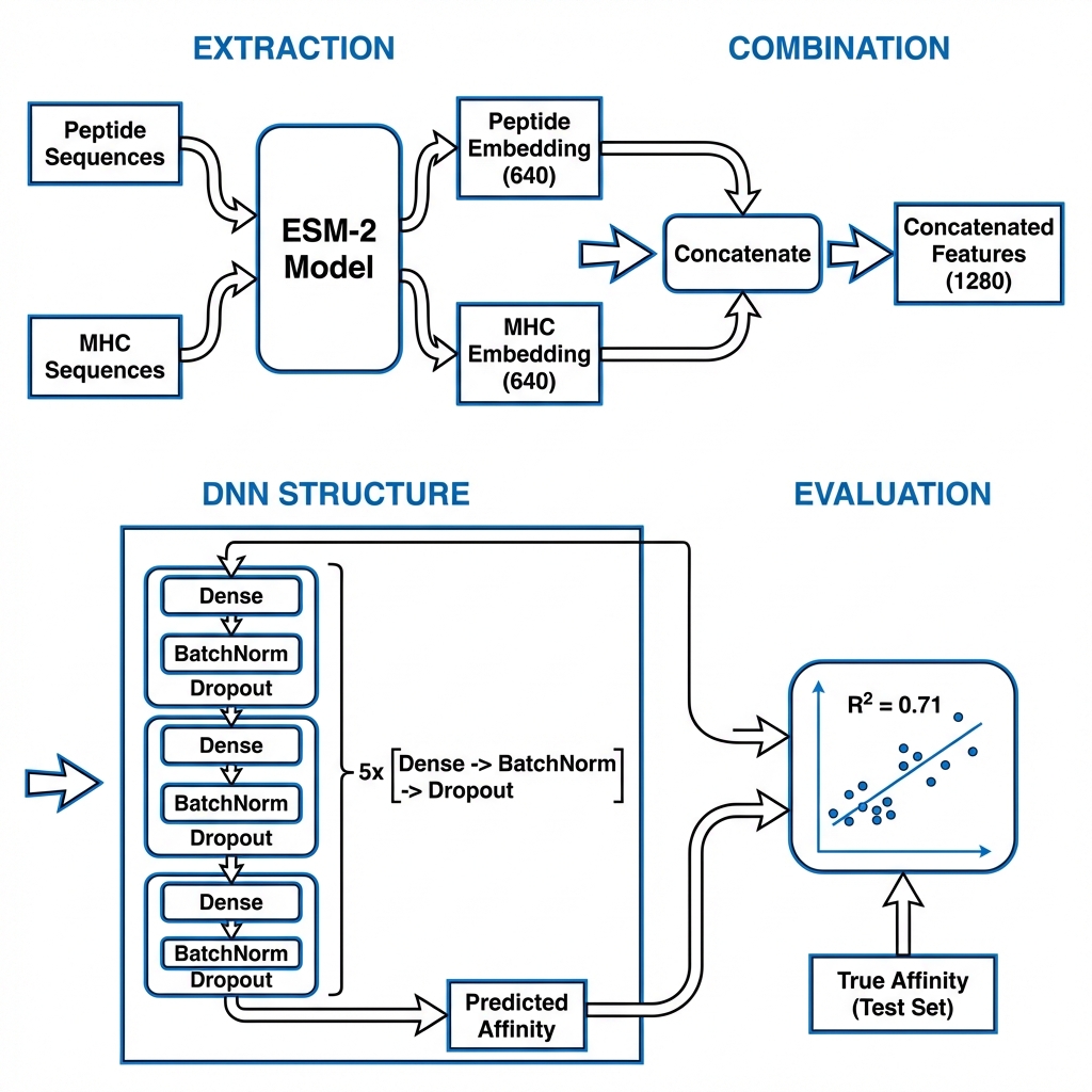
Schematic overview of the Deep Neural Network pipeline for predicting peptide-MHC binding affinity (Figure generated with the assistance of Gemini).
1. Data Selection and Splitting
We will use datasets from Therapeutics Data Commons (TDC), a large-scale data repository for machine learning projects.
Code
# Access the MHC2_IEDB_Jensen data from TDC API and obtain splitted datafrom tdc.multi_pred import PeptideMHCdata = PeptideMHC(name ="MHC2_IEDB_Jensen")split = data.get_split(method ="random", seed =524, frac = [0.7, 0.1, 0.2])train_df, valid_df, test_df = split['train'], split['valid'], split['test']
Code
# Save the files to driveimport ossave_path ='./data'os.makedirs(save_path, exist_ok=True)train_df.to_feather(os.path.join(save_path, 'train_dat.feather'))valid_df.to_feather(os.path.join(save_path, 'valid_dat.feather'))test_df.to_feather(os.path.join(save_path, 'test_dat.feather'))
2. Exploratory Data Analysis
Let’s examine the structure and distribution of our data.
Code
# how many data points in each data setprint(f"Number of data points in the training set: {len(train_df)}")print(f"Number of data points in the validation set: {len(valid_df)}")print(f"Number of data points in the test set: {len(test_df)}")
Output:
Number of data points in the training set: 93997
Number of data points in the validation set: 13428
Number of data points in the test set: 26856
A quick look at the training data reveals the structure: Peptide sequence, MHC sequence (pseudo-sequence), and the binding affinity Y.
Code
# quick look at the train data structuretrain_df.head()
Peptide
MHC
Y
MHC_ID
0
PKYVKQNTLKLAT
YAFFMF…
0.000000
HLA-DPA10103-DPB10201
1
AAAAGWQTLSAALDA
YAFFMF…
0.238910
HLA-DPA10103-DPB10201
2
AALDAQAVELTARLN
YAFFMF…
0.357937
HLA-DPA10103-DPB10201
3
ADLGYGPATPAAPAA
YAFFMF…
0.285795
HLA-DPA10103-DPB10201
4
AGSYAADLGYGPATP
YAFFMF…
0.108843
HLA-DPA10103-DPB10201
Distribution of Binding Affinity
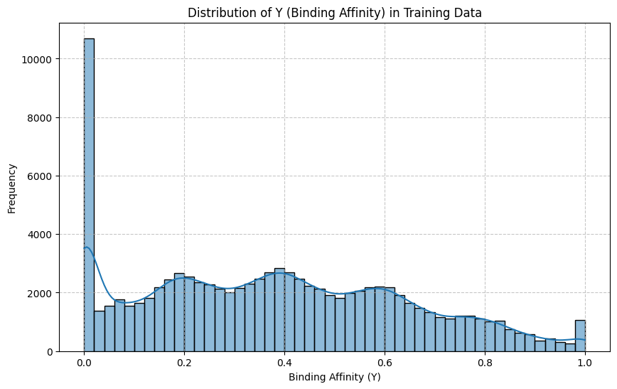
We can visualize the distribution of the target variable Y (binding affinity) in the training set.
Code
# look at the distribution of Y in training dataimport matplotlib.pyplot as pltimport seaborn as snsplt.figure(figsize=(10, 6))sns.histplot(train_df['Y'], bins=50, kde=True)plt.title('Distribution of Y (Binding Affinity) in Training Data')plt.xlabel('Binding Affinity (Y)')plt.ylabel('Frequency')plt.grid(True, linestyle='--', alpha=0.7)plt.show()
The Y values represent normalized binding affinity between the peptides and the MHC II, with higher values representing higher affinities. We can see from the distribution that many pairs have no affinity (Y = 0), while others have variable levels of affinity.
Peptide and MHC Occurrences
Code
# How many unique MHC_ID and peptides are there?unique_mhc = train_df['MHC_ID'].nunique()unique_peptides = train_df['Peptide'].nunique()print(f'Number of unique MHC_IDs in training set: {unique_mhc}')print(f'Number of unique peptides in training set: {unique_peptides}')
Output:
Number of unique MHC_IDs in training set: 79
Number of unique peptides in training set: 14597
MHC Type Distribution
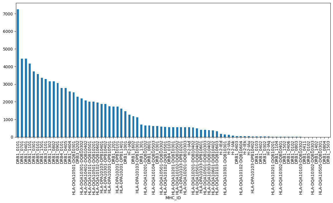
We can also look at the distribution of MHC types in our training data.
Code
# plot barplot of instances per MHC2 moleculeplt.figure(figsize=(14, 6))train_df["MHC_ID"].value_counts().sort_values(ascending =False).plot(kind ='bar')
Some MHCs have many peptide binding data points, while others have only a few. In the next session, we will remove low instance MHC data so that the prediction model has sufficient training data.
3. Extract and Merge LLM Embeddings
To represent the protein sequences for our neural network, we will use ESM-2 (Evolutionary Scale Modeling), a state-of-the-art protein language model. We’ll use the 150M parameter version (esm2_t30_150M_UR50D), which has 640 embedding dimensions.
Code
# Only keep MHC_ID that has >= 1000 instances in train data, so that the model has sufficient training datan_data = train_df["MHC_ID"].value_counts()keep_mhc_id = n_data[n_data >=1000].index.tolist()train_df = train_df[train_df["MHC_ID"].isin(keep_mhc_id)].reset_index(drop=True)valid_df = valid_df[valid_df["MHC_ID"].isin(keep_mhc_id)].reset_index(drop=True)test_df = test_df[test_df["MHC_ID"].isin(keep_mhc_id)].reset_index(drop=True)
Code
# How many data points in each data setprint(f"Number of data points in the training set: {len(train_df)}")print(f"Number of data points in the validation set: {len(valid_df)}")print(f"Number of data points in the test set: {len(test_df)}")
Output:
Number of data points in the training set: 82388
Number of data points in the validation set: 11702
Number of data points in the test set: 23410
Code
from transformers import AutoTokenizer, EsmModel# model checkpoints can be seen here: https://github.com/facebookresearch/esm#available-models-and-datasets-# the one we use has medium complexity and has 640 dimensionsmodel_checkpoint ="facebook/esm2_t30_150M_UR50D"tokenizer = AutoTokenizer.from_pretrained(model_checkpoint)model = EsmModel.from_pretrained(model_checkpoint)
A note to LLM model selection for this specific task: I’ve tried larger ESM2 model with 1280 or 2560 embedding dimensions, and they did not improve the accuracy of binding prediction. As peptides and MHC lengths are quite short, it is possible that the 640 dimension model has already saturated learnable information for this task.
Code
# Write a function to extract mean embeddings for protein sequences# GPU will significantly speed up the process# This is memory intensive, so we will batch the iterationimport numpy as npfrom transformers import AutoTokenizer, EsmModelimport torchimport mathfrom tqdm import tqdmimport pandas as pddef extract_mean_embedding( sequence: list[str], tokenizer: AutoTokenizer, model: EsmModel, device: torch.device |None=None, batch_size: int=64 ) -> pd.DataFrame:"""Extract mean embeddings for peptide sequences from a LLM model."""# Use GPU when availableifnot device: device = torch.device("cuda"if torch.cuda.is_available() else"cpu")# Separate sequence list into batches n_batches = math.ceil(len(sequence) / batch_size) all_batch_embeddings = [] model = model.to(device) # Move model to the target device model.eval() # Set model to evaluation mode steps = tqdm(range(n_batches))for i in steps: steps.set_description(f"Processing batch {i+1}/{n_batches}") start = i * batch_size end = (i +1) * batch_size batch = sequence[start:end]# Tokenize peptide sequence and pad to equal length inputs = tokenizer(batch, return_tensors="pt", padding=True)# Move input to the target device inputs = {name: tensor.to(device) for name, tensor in inputs.items()}# Forward pass through the model without gradient tracking to get mean embeddingswith torch.no_grad(): batch_mean_embeddings = model(**inputs).last_hidden_state.mean(dim=1).detach().cpu().numpy() all_batch_embeddings.append(batch_mean_embeddings) embeddings = pd.DataFrame(np.vstack(all_batch_embeddings)) embeddings.columns = [f"me_{i +1}"for i inrange(embeddings.shape[1])]return embeddings
The ESM2 model returns a sequence of embeddings for each token in the input sequence. We take the mean of these embeddings to get a single embedding for the entire sequence. It is also possible to keep the sequence of embeddings for each token, and use other methods to aggregate the embeddings, such as max pooling or attention pooling, or train a 1D Convolutional Neural Network (CNN) to learn the optimal way to aggregate the embeddings. In this case, we will keep the mean embeddings for each sequence.
Code
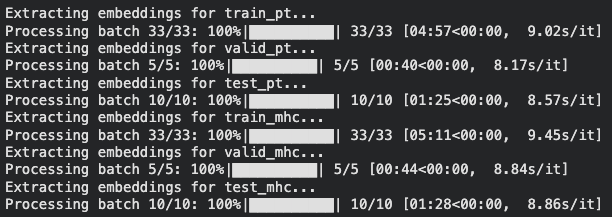
# Put all peptide/MHC data into a dictionarysequence_dict = {"train_pt": train_df['Peptide'].tolist(),"valid_pt": valid_df['Peptide'].tolist(),"test_pt": test_df['Peptide'].tolist(),"train_mhc": train_df['MHC'].tolist(),"valid_mhc": valid_df['MHC'].tolist(),"test_mhc": test_df['MHC'].tolist()}# Extract embeddings for all peptide/MHC dataembedding_dict = {}for data, sequence in sequence_dict.items():print(f"Extracting embeddings for {data}...") embedding_dict[data] = extract_mean_embedding(sequence, tokenizer, model, batch_size=2560)
There are other, more complex ways to combine embeddings from two interacting entities, but for this task, we will use the simple approach of concatenating the embeddings.
Code
# Modify column names to add peptide/MHC prefixfor key, me in embedding_dict.items(): me.columns = [f"{key.split('_')[1]}_{col}"for col in me.columns]# Concatenate peptide and MHC mean embeddings and name columnstrain_me = pd.concat([train_df[['Peptide', 'MHC_ID', 'Y']], embedding_dict['train_pt'], embedding_dict['train_mhc']], axis=1)valid_me = pd.concat([valid_df[['Peptide', 'MHC_ID', 'Y']], embedding_dict['valid_pt'], embedding_dict['valid_mhc']], axis=1)test_me = pd.concat([test_df[['Peptide', 'MHC_ID', 'Y']], embedding_dict['test_pt'], embedding_dict['test_mhc']], axis=1)# Save data as feather filesmodel_cp =str(model.name_or_path).replace('/', '_')df_list = [(train_me, 'train_me'), (valid_me, 'valid_me'), (test_me, 'test_me')]save_path ='./data'for df, df_name in df_list: df.to_feather(os.path.join(save_path, f'{model_cp}_{df_name}.feather'))
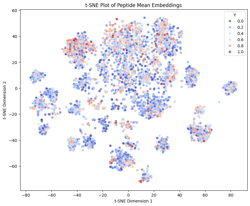
Let’s visualize the embeddings using t-SNE to see if there are any patterns in the data.
Code
# Plot t-SNE of sampled peptide-MHC mean embeddingsimport matplotlib.pyplot as pltimport seaborn as snsfrom sklearn.manifold import TSNEsampled_index = train_me.sample(n=5000, random_state=1).index # sample 5000 data points for visualizationX_embedded = TSNE(n_components=2, learning_rate='auto', init='random', perplexity=30).fit_transform(train_me.loc[sampled_index])plt.figure(figsize=(10, 8))plt.scatter(X_embedded[:, 0], X_embedded[:, 1], alpha=0.5, s=2)plt.title('t-SNE of Peptide-MHC Embeddings')plt.show()
In the above t-SNE plot, we can see some cluster structures correlating with higher Y, indicating that the embeddings encode information relating to peptide-MHC affinity.
4. Neural Network Training
We will build a MLP that takes the concatenated peptide and MHC embeddings as input, and outputs the predicted affinity.
Dataset Preparation
We convert our extracted embeddings and labels into TensorFlow datasets.
Code
# Convert data to Tensorflow datasetimport tensorflow as tfimport pandas as pd# Compile all feature columns (peptide and MHC embeddings) into a single NumPy array for each datasetX_train = train_me.filter(regex=f"^pt|^mhc").valuesy_train = train_me['Y'].valuesX_valid = valid_me.filter(regex=f"^pt|^mhc").valuesy_valid = valid_me['Y'].valuesX_test = test_me.filter(regex=f"^pt|^mhc").valuesy_test = test_me['Y'].values# Create tf.data.Dataset from these concatenated arraystrain_tfds = tf.data.Dataset.from_tensor_slices((X_train, y_train))# Shuffle, batch and prefetch the tfdstrain_tfds = train_tfds.shuffle(1024, seed=42).batch(32).prefetch(1)valid_tfds = tf.data.Dataset.from_tensor_slices((X_valid, y_valid))valid_tfds = valid_tfds.batch(32).prefetch(1)
Model Architecture
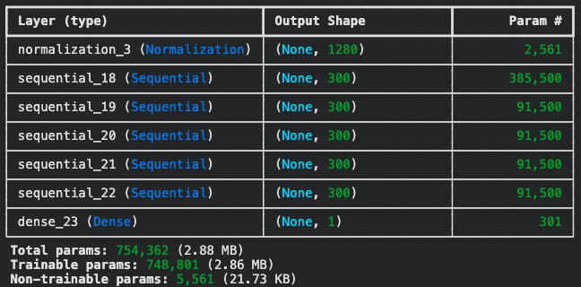
The model consists of dense layers with varying dropout rates to prevent overfitting.
Code
# Define MLP layers# Define a helper function for the repetitive dense -> batch norm -> dropout blockdef make_dense_block(n_neurons, dropout_rate=0.2):return tf.keras.Sequential([ tf.keras.layers.Dense(n_neurons, activation='relu', kernel_initializer='he_normal'), tf.keras.layers.BatchNormalization(), tf.keras.layers.Dropout(dropout_rate) ])tf.random.set_seed(42)norm_layer = tf.keras.layers.Normalization(input_shape=X_train.shape[1:])dnn_model = tf.keras.Sequential([ norm_layer, make_dense_block(300), make_dense_block(300), make_dense_block(300), make_dense_block(300), make_dense_block(300), tf.keras.layers.Dense(1)])dnn_model.summary()
Here I am using a MLP of 5 layers, with batch normalization and dropout after each layer to control for overfitting.
Training
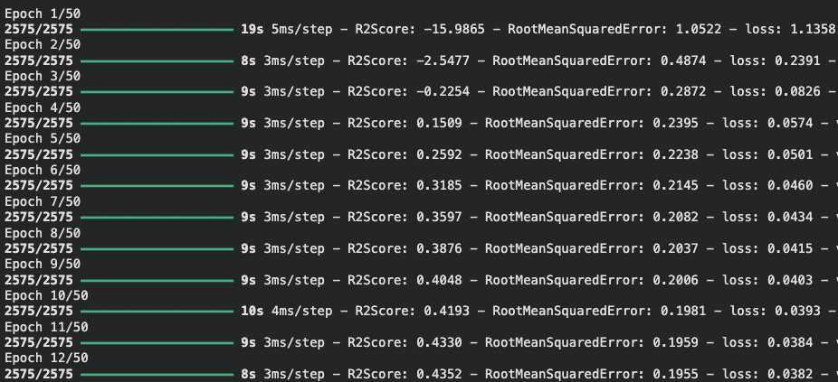
I used performance scheduling to make sure that the model converges to a good solution. I also used early stopping to further prevent overfitting.
Code
# Performance scheduling of learning ratelr_scheduler = tf.keras.callbacks.ReduceLROnPlateau(factor=0.5, patience=5)# Early stoppingearly_stopping = tf.keras.callbacks.EarlyStopping(patience=10, restore_best_weights=True)
Code
optimizer = tf.keras.optimizers.Adam(learning_rate=1e-4)dnn_model.compile(loss='mse', optimizer=optimizer, metrics=['RootMeanSquaredError', 'R2Score'])# Adapt the normalization layer using only the feature tensors from the datasetnorm_layer.adapt(train_tfds.map(lambda x, y: x))tf.random.set_seed(42)fit_history = dnn_model.fit(train_tfds, epochs=50, validation_data=valid_tfds, callbacks=[lr_scheduler, early_stopping])
Training History
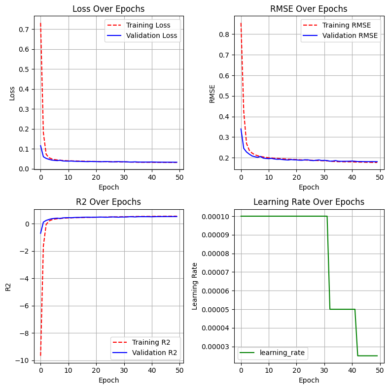
Let’s analyze the training performance over epochs.
Code
# Plot train and validation loss and RMSE across epochsimport matplotlib.pyplot as pltfig, ax = plt.subplots(nrows=2, ncols=2, figsize=(8, 8))pd.DataFrame(fit_history.history)[['loss', 'val_loss']].plot( grid=True, xlabel="Epoch", ax=ax[0, 0], style=["r--", "b-"])pd.DataFrame(fit_history.history)[['RootMeanSquaredError', 'val_RootMeanSquaredError']].plot( grid=True, xlabel="Epoch", ax=ax[0, 1], style=["r--", "b-"])pd.DataFrame(fit_history.history)[['R2Score', 'val_R2Score']].plot( grid=True, xlabel="Epoch", ax=ax[1, 0], style=["r--", "b-"])pd.DataFrame(fit_history.history)[['learning_rate']].plot( grid=True, xlabel="Epoch", ax=ax[1, 1], style=["g-"])ax[0, 0].set_ylabel('Loss')ax[0, 0].set_title('Loss Over Epochs')ax[0, 0].legend(['Training Loss', 'Validation Loss'])ax[0, 1].set_ylabel('RMSE')ax[0, 1].set_title('RMSE Over Epochs')ax[0, 1].legend(['Training RMSE', 'Validation RMSE'])ax[1, 0].set_ylabel('R2')ax[1, 0].set_title('R2 Over Epochs')ax[1, 0].legend(['Training R2', 'Validation R2'])ax[1, 1].set_ylabel('Learning Rate')ax[1, 1].set_title('Learning Rate Over Epochs')plt.tight_layout()plt.show()
As we can see, validation loss and errors have been kept very close to that of training, and they eventually dropped down to very similar levels, suggesting that the model did not overfit.
5. Model Evaluation
Finally, we evaluate the model on the training and test set.
Training Set
Code
# Evaluate R-squared of predicted vs actual binding affinity for each MHC typefrom sklearn.metrics import r2_scorey_pred = dnn_model.predict(X_train)y_true = y_trainmhc_id = train_me['MHC_ID'].valuesr2_df = pd.DataFrame({'MHC_ID': mhc_id, 'Y': y_true, 'Y_pred': y_pred.flatten()})# remove MHC_ID <= 10 instancesr2_df = r2_df.groupby('MHC_ID').filter(lambda x: len(x) >10)# Calculate R2 and MHC instancesmhc_n = r2_df['MHC_ID'].value_counts()r2_by_mhc = r2_df.groupby('MHC_ID').apply(lambda x: r2_score(x['Y'], x['Y_pred']))# Join statistics by MHC_IDr2_df = pd.concat([mhc_n, r2_by_mhc], axis=1)r2_df.columns = ['n', 'r2']r2_df.sort_values(by='r2', ascending=False, inplace=True)
Code
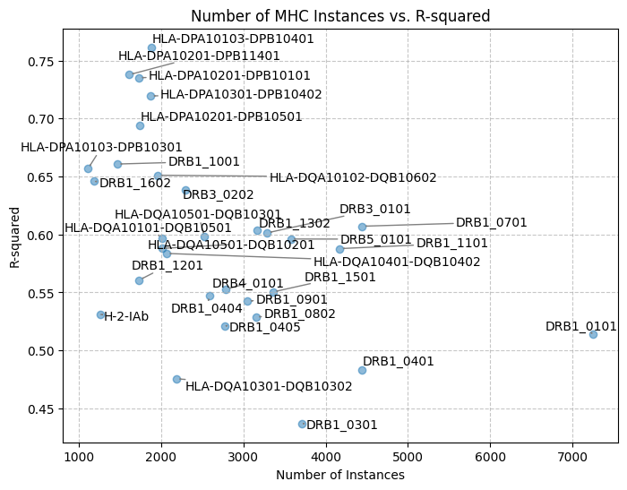
# Plot MHC instance vs prediction accuracy scatter plotplt.figure(figsize=(8, 6))plt.scatter(r2_df['n'], r2_df['r2'], alpha=0.5)from adjustText import adjust_texttexts = [plt.text(r2_df['n'].iloc[i], r2_df['r2'].iloc[i], r2_df.index[i]) for i inrange(len(r2_df))]adjust_text( texts, expand=(1.1, 1.1), arrowprops=dict(arrowstyle="->", color="grey"))plt.xlabel('Number of Instances')plt.ylabel('R-squared')plt.title('Number of MHC Instances vs. R-squared')plt.grid(True, linestyle='--', alpha=0.7)plt.show()
This plot reveals two key findings: (1) Prediction accuracy does not correlate with the number of MHC instances, suggesting that the model’s performance is driven more by the intrinsic biochemical or structural properties of the peptide-MHC pairs than by data volume. Indeed, the model did not necessarily perform better on MHCs that were abundant in the training data (e.g., DRB-0101 is very abundant yet has a relatively low \(R^2\)). (2) Some MHC interactions are inherently easier to predict. For example, HLA-DPA10201-DPB10101 achieves an \(R^2\) > 0.7. This reinforces the idea that intrinsic properties—or potentially higher-quality experimental data for these specific alleles—are the primary drivers of prediction success.
Test Set
Code
# Evaluate performance on test datadnn_model.evaluate(X_test, y_test)
The test RMSE and loss are very close to the training data and even a little better than the validation data, suggesting that the model did not overfit too much.
Code
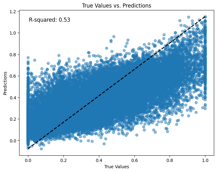
# Plot scatter plot of predicted vs actual on test dataimport matplotlib.pyplot as plty_pred = dnn_model.predict(X_test)y_true = y_testplt.figure(figsize=(8, 6))plt.scatter(y_true, y_pred, alpha=0.5)plt.plot([min(y_true), max(y_true)], [min(y_pred), max(y_pred)], 'k--', lw=2)plt.xlabel('True Values')plt.ylabel('Predictions')plt.title('True Values vs. Predictions')# Add R-squared on the plotfrom sklearn.metrics import r2_scorer2 = r2_score(y_true, y_pred)plt.text(0.05, 0.95, f'R-squared: {r2:.2f}', transform=plt.gca().transAxes, fontsize=12, verticalalignment='top')plt.show()
Overall prediction accuracy is good (\(R^2 \approx 0.53\)). However, aggregate metrics can hide specific strengths. Let’s break down performance by MHC type.
Performance by MHC Type in Test Set
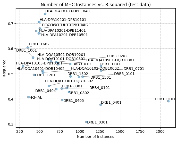
We calculate the \(R^2\) score specifically for each MHC allele in the test set (filtering for those with >10 instances).
Code
# Evaluate R-squared of predicted vs actual binding affinity for each MHC type (test data)y_pred = dnn_model.predict(X_test)y_true = y_test# ...code abbreviated for brevity...
Similar to the training set, we can see that prediction accuracy does not correlate with the number of MHC instances, and some MHCs are just easier to predict than others.
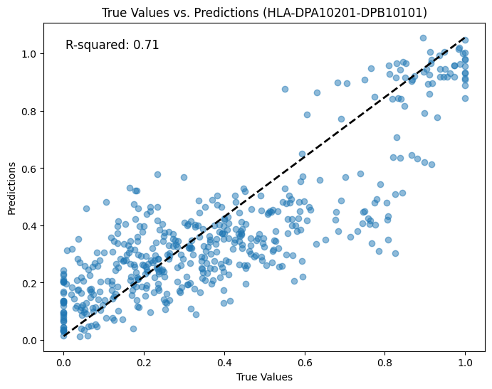
For example, looking at HLA-DPA10201-DPB10101:
Code
# Plot HLA-DPA10201-DPB10101 and peptide binding predicted vs actual scatter plotimport matplotlib.pyplot as plty_pred = dnn_model.predict(X_test)y_true = y_testmhc_id = test_me['MHC_ID'].valuestarget_mhc ='HLA-DPA10201-DPB10101'target_index = np.where(mhc_id == target_mhc)[0]y_pred = y_pred[target_index]y_true = y_true[target_index]plt.figure(figsize=(8, 6))plt.scatter(y_true, y_pred, alpha=0.5)plt.plot([min(y_true), max(y_true)], [min(y_pred), max(y_pred)], 'k--', lw=2)plt.xlabel('True Values')plt.ylabel('Predictions')plt.title('True Values vs. Predictions (HLA-DPA10201-DPB10101)')# Add R-squared on the plotfrom sklearn.metrics import r2_scorer2 = r2_score(y_true, y_pred)plt.text(0.05, 0.95, f'R-squared: {r2:.2f}', transform=plt.gca().transAxes, fontsize=12, verticalalignment='top')plt.show()
For this specific MHC type, the \(R^2\) is 0.71, which is significantly better than the global average. This demonstrates that for certain alleles, the model can reliably identify high-affinity binders (e.g., a predicted affinity cutoff of > 0.6 corresponds well to high actual affinity).
Conclusion
By leveraging ESM2 embeddings and MLP, we built a pipeline to predict peptide-MHC II binding. This exercise showcases the potential of combining LLMs with machine learning to tackle complex biological challenges. These could range from predicting protein-protein interactions and drug-target binding to forecasting drug responses from gene expression data.