Evaluating Data Leakage in Protein Binding Affinity Prediction

Research Impact

Data leakage is a critical issue in machine learning, especially in the context of protein-protein interaction (PPI) prediction. Data leakage occurs when information from the training data is inadvertently used in the testing phase, allowing the model to “remember” specific examples rather than learning generalizable patterns. To address this issue, this post compares two data splitting strategies, regular C3 split and strict C3 split, to evaluate the extent of data leakage when using pre-trained protein large language models (pLLMs) to predict peptide-MHC2 binding. The findings showed that while the neural network model generalized well on predicting binding peptides of seen MHC2 alleles, it struggled to generalize to unseen MHC2 alleles. This highlights the importance of using strict data splitting strategies to ensure that models are evaluated on truly unseen data, which is crucial for developing robust and generalizable models in protein binding affinity prediction.

Introduction

I’ve recently come across this paper about data leakage in PPI prediction models using pLLMs, and it got me thinking about how data leakage might affect other types of protein interaction predictions, such as peptide-MHC2 binding. In this project, I decided to explore this issue by comparing two different data splitting strategies: a regular C3 split and a strict C3 split. The regular C3 split allows for some overlap between the training and testing sets, while the strict C3 split ensures that there is no overlap at all. By evaluating the performance of a neural network model trained on embeddings extracted from a pre-trained pLLM (ESM2) under these two splitting strategies, I aimed to understand the extent of data leakage and its impact on model generalization in the context of peptide-MHC2 binding prediction.

Key Steps

1. Splitting Strategies: Peptide or MHC sequences were first clustered independently using two different approaches. In both cases, the goal was to ensure that similar protein sequences were not present in both the training and testing sets. Peptides were clustered based on a 3-gram sequence similarity approach, while MHC pseudo-sequences were clustered based on their BLOSUM62 amino acid similarity. After that, the cluster classes were split into training and testing sets using two different strategies largely based on the C3 approach:

   • Regular C3 split: This split ensures that the test set contains pairs \((Peptide_{new}, MHC_{any})\) and \((Peptide_{any}, MHC_{new})\). This is a less strict C3 split, as it allows for some overlap in the individual components (peptides and MHCs) between the training and testing sets, but not in the interactions.

   • Strict C3 split: This split ensures that for every pair \((Peptide, MHC)\) in the test set, both \(Peptide\) and \(MHC\) classes are entirely absent from the training set. This is the “Double-Cold” strategy, which is more stringent and ensures that the model is evaluated on completely unseen peptides and MHCs, thus providing a more accurate assessment of the model’s generalization capabilities. A down side of this split is that it results in a smaller training and testing set. To ensure a fair comparison between the two splits, the sample number from the “regular C3 split” was downsampled to match the sample number from the “strict C3 split”.

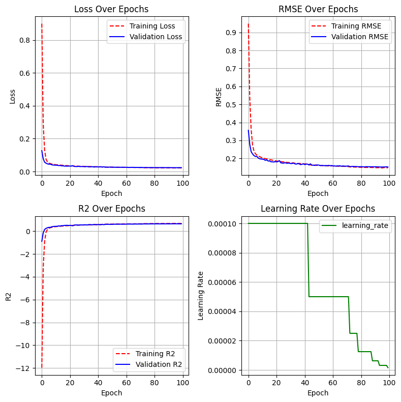
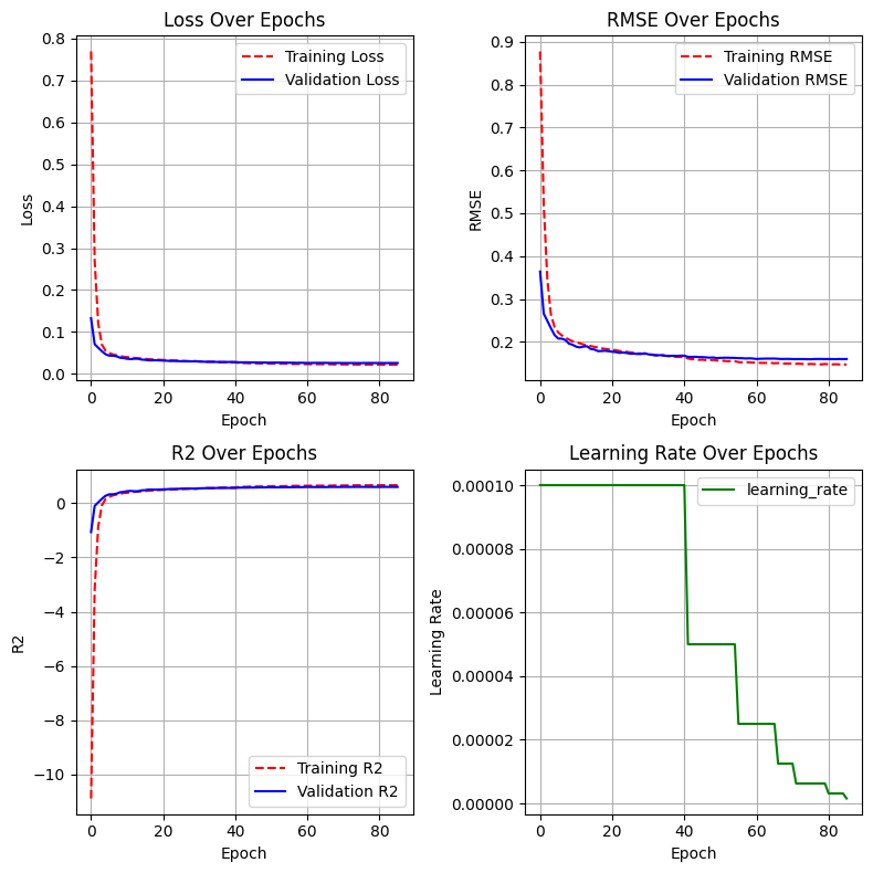
2. Embeddings Extraction and Model Training: Similar to my previous post, we will extract ESM2 embeddings for both peptides and MHC2 pseudo-sequences. The embeddings will be extracted in a way that retains the 2D structure, which is crucial for applying convolutional layers in the model. After extracting the embeddings, we will concatenate the peptide and MHC2 embeddings along the sequence length dimension, retaining the sequence information and the 2D structure. We will then define a model architecture that includes two 1D convolutional layers followed by a self-attention layer and five dense layers. The model will be trained separately on the datasets generated from the regular C3 split and the strict C3 split, allowing us to compare the performance of the model under both splitting strategies.

3. Comparing Regular vs. Strict C3 split: After training the model on both datasets, we will evaluate its performance using appropriate metrics such as \(R^2\) score, root mean squared error (RMSE), and loss.

1. Data Splitting Strategies

Loading required libraries:

import pandas as pd
import numpy as np
from sklearn.cluster import AgglomerativeClustering
from sklearn.model_selection import GroupShuffleSplit
from Bio.Align import substitution_matrices
from sklearn.feature_extraction.text import CountVectorizer
from sklearn.metrics.pairwise import cosine_similarity
from sklearn.model_selection import train_test_split

See my previous post for source of data. First, let’s see what the input data looks like:

df.head()

Output:

   Peptide_ID           Peptide     MHC_ID  \
0      104653   VAPIEHIASMRRNYF  DRB1_1302   
1       37106   HDDKETSFIRNCARK  DRB1_0101   
2      118433   LIWVGINTRNMTMSM  DRB1_0101   
3       80770  GVTVIKNNMINNDLGP  DRB1_1501   
4       19888   PAPMLAAAAGWQTLS  DRB1_1101   

                                  MHC         Y  
0  QEFFIASGAAVDAIMESSFDYFDIDEATYHVGFT  0.501084  
1  QEFFIASGAAVDAIMWLFLECYDLQRATYHVGFT  0.441298  
2  QEFFIASGAAVDAIMWLFLECYDLQRATYHVGFT  0.217673  
3  QEFFIASGAAVDAIMWPRFDYFDIQAATYHVVFT  0.807811  
4  QEFFIASGAAVDAIMESSFDYFDFDRATYHVGFT  0.583271  

Here we have the peptide sequences, MHC pseudo-sequences, and their corresponding binding affinity values (Y).

Let’s perfrom peptide clustering using a 3-gram approach to find overlapping peptides without source information. We will use the CountVectorizer from sklearn to create a matrix of 3-gram counts for each unique peptide, and then compute the cosine similarity between the peptides based on this matrix. Finally, we will use hierarchical clustering to group similar peptides together.

vect = CountVectorizer(analyzer='char', ngram_range=(3, 3)) # sequence of 3 a.a.
pep_matrix = vect.fit_transform(df['Peptide'].unique()) # row: unique peptides, col: unique 3 a.a.
pep_sim = cosine_similarity(pep_matrix) # peptide X peptide similarity matrix
# use cosine dist when the orientation or pattern of the data is more important than the absolute scale
# often used in text, genetic sequence

# Cluster peptides that share many 3-mers (likely from the same protein)
pep_clusters = AgglomerativeClustering(
    n_clusters=None,
    distance_threshold=0.5, # Adjust: lower = more groups, stricter split
    metric='precomputed', # input is pre-computed dist
    linkage='complete'
).fit_predict(1 - pep_sim)

pep_map = pd.DataFrame({
    'Peptide': df['Peptide'].unique(),
    'pep_group': pep_clusters
})

df = df.merge(pep_map, on='Peptide')

print(pep_map.sort_values(by='pep_group').head(15))

Output:

                    Peptide  pep_group
1576         QYIKANAKFIGITE          0
702       YATFFIKANSKFIGITE          0
6842       MQYIKANSKFIGITEL          0
15556        QYQKANSKFIGITE          0
4185         QYIKANSKFIGITE          0
7940   SAMILAAYHPQQFIYAGSLS          1
16944  AAIGLSMAGSSAMILAAYHP          1
9611       RQIRMAKLLGRDPEQS          2
860        HGRQIRMAKLFGRDPE          2
6826       EGELHGRQIRMAKLLG          2
14166      HGRQIKMAKLLGRDPE          2
687         HGRQIRMAKLLGRDP          2
4640       HGRQIRMAKLLGRDPE          2
6532       HGRQIRMAKLLTRDPE          2
4614        QIRMAKLLGRDPEQS          2

We can see that peptides that are likely from the same protein (e.g., “QYIKANAKFIGITE”, “YATFFIKANSKFIGITE”, “MQYIKANSKFIGITEL”) are clustered together in the same group (group 0). This indicates that our clustering approach is effectively grouping similar peptides together based on their 3-gram composition.

Next, we will cluster MHC pseudo-sequences based on their BLOSUM62 amino acid similarity. We will define a function to calculate the BLOSUM62 similarity between two sequences, and then create a similarity matrix for the MHC pseudo-sequences. Finally, we will use hierarchical clustering to group similar MHCs together.

# Function to calculate BLOSUM62 similarity
def blosum62_similarity(seq1, seq2):
    matrix = substitution_matrices.load('BLOSUM62')
    score = 0.0

    # Align sequences by padding the shorter one (simple padding for score calculation)
    # Note: For rigorous alignment, a proper sequence alignment algorithm (e.g., Needleman-Wunsch) is needed.
    # This simplified approach assumes aligned positions are comparable.
    for i in range(min(len(seq1), len(seq2))):
        try:
            score += matrix[seq1[i], seq2[i]]
        except KeyError: # Handle cases where amino acid might not be in BLOSUM (e.g., 'X')
            score += 0 

    # Normalize score (for simplicity, divide by max possible score)
    # A more robust normalization might involve the self-similarity score.
    # Here a max possible similarity score for each aa is calculated and summed
    max_score1 = sum(matrix[aa, aa] for aa in seq1 if (aa, aa) in matrix.keys())
    max_score2 = sum(matrix[aa, aa] for aa in seq2 if (aa, aa) in matrix.keys())
    if max_score1 == 0 or max_score2 == 0: # Avoid division by zero
        return 0.0
    return score / max(max_score1, max_score2)

mhc_sequences = df['MHC'].unique()

# Create a similarity matrix for MHCs
n_mhc = len(mhc_sequences)
mhc_sim_matrix = np.zeros((n_mhc, n_mhc))
for i in range(n_mhc):
    for j in range(i, n_mhc):
        sim = blosum62_similarity(mhc_sequences[i], mhc_sequences[j])
        mhc_sim_matrix[i, j] = sim
        mhc_sim_matrix[j, i] = sim

# Cluster MHCs
mhc_clusters = AgglomerativeClustering(
    n_clusters=None,
    distance_threshold=0.2, # Adjust: lower = more groups, stricter split for MHCs
    metric='precomputed',
    linkage='complete'
).fit_predict(1 - mhc_sim_matrix)

mhc_map = pd.DataFrame({
    'MHC': mhc_sequences,
    'mhc_group': mhc_clusters
})

df = df.merge(mhc_map, on='MHC')

print(mhc_map.sort_values(by='mhc_group'))

Output:

                                   MHC  mhc_group
5   QEFFIASGAAVDAIMELSFEYYVLQKQNYHVVFT          0
15  QEFFIASGAAVDAIMERSYDYYVLQKRNYHVGFT          0
12  QEFFIASGAAVDAIMELSFEHYDLQKQNYHVGFT          0
8   QEFFIASGAAVDAIMESSYDYFDLQKRNYHVVFT          0
9   CNYHQGGGARVAHIMFFGLTYYDVGTETVHVAGI          1
..                                 ...        ...
64  YTYFLRRGGQTGHILHFPLIYYDYRTETVHKTPT         26
66  XXYHWTSGGQTGHGWALGSNYYDIRTETVHGVHT         27
70  QEFFIASGAAVDAIMESSFEYYDLQRATYHVGFT         28
62  QEFFIASGAAVDAIMESSFEYYDLQKRNYHVGFT         28
29  QEFFIASGAAVDAIMESGLEHFVIDRATYHAVFT         29

[75 rows x 2 columns]

We can see that MHC pseudo-sequences that are similar based on their BLOSUM62 scores are clustered together in the same group (e.g., “QEFFIASGAAVDAIMELSFEYYVLQKQNYHVVFT”, “QEFFIASGAAVDAIMERSYDYYVLQKRNYHVGFT”, “QEFFIASGAAVDAIMELSFEHYDLQKQNYHVGFT” are all in group 0). This indicates that our clustering approach is effectively grouping similar MHC pseudo-sequences together based on their amino acid composition and similarity.

Next, we will perform the regular C3 split. To ensure total isolation between the training and testing sets, we will create a ‘SuperGroup’ that combines both the peptide and MHC groups. This way, we can ensure that no similar peptide-MHC pairs are present in both the training and testing sets, thus minimizing data leakage.

# Perform the "Regular C3 split" first
# We create a 'SuperGroup' that combines both to ensure total isolation
df['super_group'] = df['pep_group'].astype(str) + "_" + df['mhc_group'].astype(str)

# Split train vs temp_test
gss = GroupShuffleSplit(n_splits=1, train_size=0.7, random_state=42)
train_indices, temp_test_indices = next(gss.split(df, groups=df['super_group']))

train_df = df.iloc[train_indices][['Peptide_ID', 'Peptide', 'MHC_ID', 'MHC', 'Y']]
temp_test_df = df.iloc[temp_test_indices]

# Split temp_text into test and valid
gss1 = GroupShuffleSplit(n_splits=1, train_size=0.66, random_state=42)
test_indices, valid_indices = next(gss1.split(temp_test_df, groups=temp_test_df['super_group']))

test_df = df.iloc[test_indices][['Peptide_ID', 'Peptide', 'MHC_ID', 'MHC', 'Y']]
valid_df = df.iloc[valid_indices][['Peptide_ID', 'Peptide', 'MHC_ID', 'MHC', 'Y']]

print(df)

Output:

        Peptide_ID               Peptide                 MHC_ID  \
0            29993       MSGPMQQLTQPLQQV  HLA-DPA10201-DPB11401   
1            50950  CGKYLFNWAVRTKLKLTPIA              DRB1_1302   
2            58992       YKRQLMNILGAVYRY  HLA-DPA10201-DPB10101   
3             8140       FLGCLVKEIPPRLLY  HLA-DQA10501-DQB10201   
4           111514       KTQIDQVESTAGSLQ  HLA-DPA10201-DPB10501   
...            ...                   ...                    ...   
134276       15592       RFFLPIFSEFVLLAT              DRB1_0405   
134277       21667      EVFFQRLGIASGRARY              DRB1_1302   
134278       62271       YLFAKDKSGPLQPGV  HLA-DQA10102-DQB10602   
134279       79102       GELQIVDKIDADFKI              DRB1_1302   
134280      100096       SAAPLRTITADTFRK              DRB1_0701   

                                       MHC         Y  pep_group  mhc_group  \
0       YAFFQFSGGAILNTLHLQFEYFDLEKVRVHLDVT  0.216969       6334          6   
1       QEFFIASGAAVDAIMESSFDYFDIDEATYHVGFT  0.559077        205          3   
2       YAFFQFSGGAILNTLYGQFEYFAIEKVRVHLDVT  0.423504        457          6   
3       YNYHQRXFATVLHSLYFGLSSFAIRKARVHLETT  0.328660       1876         21   
4       YAFFQFSGGAILNTLFGQFEYFEIEKVRMHLDVT  0.000000       1157          6   
...                                    ...       ...        ...        ...   
134276  QEFFIASGAAVDAIMEVHFDYYSLQRATYHVGFT  0.721843       6951          4   
134277  QEFFIASGAAVDAIMESSFDYFDIDEATYHVGFT  0.257618       3632          3   
134278  CNYHQGGGARVAHIMFFGLTYYDVGTETVHVAGI  0.141380       2158          1   
134279  QEFFIASGAAVDAIMESSFDYFDIDEATYHVGFT  0.409599       3568          3   
134280  QEFFIASGAAVDAIMWGYFELYVIDRQTVHVGFT  0.242001       1440         17   

       super_group  
0           6334_6  
1            205_3  
2            457_6  
3          1876_21  
4           1157_6  
...            ...  
134276      6951_4  
134277      3632_3  
134278      2158_1  
134279      3568_3  
134280     1440_17  

[134281 rows x 8 columns]

Now, let’s perform the strict C3 split. In this split, we will ensure that for every pair \((Peptide, MHC)\) in the test set, both the peptide and MHC classes are entirely absent from the training set. This means that we will first split the MHC groups and then split the peptide groups independently, ensuring that there is no overlap in either component between the training and testing sets.

def strict_double_split(df, train_size=0.7):
    # 1. First, split the MHC groups
    gss_mhc = GroupShuffleSplit(n_splits=1, train_size=train_size, random_state=42)
    mhc_train_idx, mhc_test_idx = next(gss_mhc.split(df, groups=df['mhc_group']))
    
    mhc_train_alleles = df.iloc[mhc_train_idx]['mhc_group'].unique()
    mhc_test_alleles = df.iloc[mhc_test_idx]['mhc_group'].unique()
    
    # 2. Second, split the Peptides groups
    # This prevents the model from seeing different fragments of the same protein
    gss_pep = GroupShuffleSplit(n_splits=1, train_size=train_size, random_state=42)
    pep_train_idx, pep_test_idx = next(gss_pep.split(df, groups=df['pep_group']))
    
    pep_train_prots = df.iloc[pep_train_idx]['pep_group'].unique()
    pep_test_prots = df.iloc[pep_test_idx]['pep_group'].unique()
    
    # 3. Create the "Strict" Test Set: 
    # Only interactions where BOTH the MHC is new AND the Protein is new.
    train_df = df[df['mhc_group'].isin(mhc_train_alleles) & df['pep_group'].isin(pep_train_prots)].copy()
    test_df = df[df['mhc_group'].isin(mhc_test_alleles) & df['pep_group'].isin(pep_test_prots)].copy()
    
    return train_df, test_df

train_temp, test_strict = strict_double_split(df)

# Random split of data into train or valid data
train_strict, valid_strict = train_test_split(train_temp, test_size=0.125, random_state=42)

# Save data to disc
import os
save_path = '/data'
train_df.to_feather(os.path.join(save_path, 'train_dat_cold.feather'))
valid_df.to_feather(os.path.join(save_path, 'valid_dat_cold.feather'))
test_df.to_feather(os.path.join(save_path, 'test_dat_cold.feather'))
train_strict.to_feather(os.path.join(save_path, 'train_dat_strict.feather'))
valid_strict.to_feather(os.path.join(save_path, 'valid_dat_strict.feather'))
test_strict.to_feather(os.path.join(save_path, 'test_dat_strict.feather'))

train_df.shape, test_df.shape, valid_df.shape
train_strict.shape, test_strict.shape, valid_strict.shape

Output:

Regular split shape:
((93392, 5), (26531, 5), (14358, 5))

Strict split shape:
((59757, 8), (9588, 8), (8537, 8))

We can see that the regular C3 split results in a larger training and testing set compared to the strict C3 split. When we prepare the data for model training, we will need to downsample the regular C3 split to match the sample size of the strict C3 split to ensure a fair comparison between the two splitting strategies.

2. Embeddings Extraction and Model Training

Embedding extraction and model training procedures are similar to my previous post, so I will not go through the code in detail here. Let’s load the data and downsample the regular C3 split to match the sample size of the strict C3 split:

all_dat = {
    'train': pd.read_feather(os.path.join(load_path, 'train_dat_cold.feather')).sample(n=59757, random_state=42).reset_index(drop=True), 
    'valid': pd.read_feather(os.path.join(load_path, 'valid_dat_cold.feather')).sample(n=8537, random_state=42).reset_index(drop=True),
    'test': pd.read_feather(os.path.join(load_path, 'test_dat_cold.feather')).sample(n=9588, random_state=42).reset_index(drop=True)
}

# Shuffle samples
for keys, df in all_dat.items():
  all_dat[keys] = df.sample(frac=1, random_state=42).reset_index(drop=True)

For both data splits, we will extract ESM2 embeddings (facebook/esm2_t30_150M_UR50D) for the peptides and MHC pseudo-sequences, concatenate them, and then train a neural network model with convolutional layers. The model architecture and training procedure will be the same for both splits.

Here is the model architecture we will use:

# Define 1D CNN + attention + MLP with multiple inputs using functional API
import tensorflow as tf
tf.keras.backend.clear_session()

tf.random.set_seed(42)

def make_dense_block(n_neurons, dropout_rate=0.2):
    return tf.keras.Sequential([
        tf.keras.layers.Dense(n_neurons, activation='relu', kernel_initializer='he_normal'),
        tf.keras.layers.BatchNormalization(),
        tf.keras.layers.Dropout(dropout_rate)
    ])

# Define the input layers
embedding_input = tf.keras.layers.Input(shape=embedding_dict['train'].shape[1:], name='embedding_input')
peptide_length_input = tf.keras.layers.Input(shape=(1,), name='peptide_length_input')
mhc_length_input = tf.keras.layers.Input(shape=(1,), name='mhc_length_input')

# CNN branch for embeddings
x = tf.keras.layers.Conv1D(filters=128, kernel_size=5, padding='same', activation='relu')(embedding_input)
x = tf.keras.layers.BatchNormalization()(x)
x = tf.keras.layers.Dropout(0.2)(x)
x = tf.keras.layers.Conv1D(filters=64, kernel_size=3, padding='same', activation='relu')(x)
x = tf.keras.layers.BatchNormalization()(x)
x = tf.keras.layers.Dropout(0.2)(x)
x = tf.keras.layers.AveragePooling1D(pool_size=2)(x)

# Self-attention layer
attention_output = tf.keras.layers.Attention()([x, x])
flat_attention = tf.keras.layers.Flatten()(attention_output)

# Concatenate attention output with length inputs
combined_features = tf.keras.layers.Concatenate()([flat_attention, peptide_length_input, mhc_length_input])

# MLP branch
y = make_dense_block(128)(combined_features)
y = make_dense_block(128)(y)
y = make_dense_block(128)(y)
y = make_dense_block(128)(y)
y = make_dense_block(128)(y)
output = tf.keras.layers.Dense(1)(y)

# Create the functional model
cnn_model = tf.keras.Model(inputs=[embedding_input, peptide_length_input, mhc_length_input], outputs=[output])

cnn_model.summary()

 Model: "functional_5"

┏━━━━━━━━━━━━━━━━━━━━━┳━━━━━━━━━━━━━━━━━━━┳━━━━━━━━━━━━┳━━━━━━━━━━━━━━━━━━━┓
┃ Layer (type)        ┃ Output Shape      ┃    Param # ┃ Connected to      ┃
┡━━━━━━━━━━━━━━━━━━━━━╇━━━━━━━━━━━━━━━━━━━╇━━━━━━━━━━━━╇━━━━━━━━━━━━━━━━━━━┩
│ embedding_input     │ (None, 71, 640)   │          0 │ -                 │
│ (InputLayer)        │                   │            │                   │
├─────────────────────┼───────────────────┼────────────┼───────────────────┤
│ conv1d (Conv1D)     │ (None, 71, 128)   │    409,728 │ embedding_input[… │
├─────────────────────┼───────────────────┼────────────┼───────────────────┤
│ batch_normalization │ (None, 71, 128)   │        512 │ conv1d[0][0]      │
│ (BatchNormalizatio… │                   │            │                   │
├─────────────────────┼───────────────────┼────────────┼───────────────────┤
│ dropout (Dropout)   │ (None, 71, 128)   │          0 │ batch_normalizat… │
├─────────────────────┼───────────────────┼────────────┼───────────────────┤
│ conv1d_1 (Conv1D)   │ (None, 71, 64)    │     24,640 │ dropout[0][0]     │
├─────────────────────┼───────────────────┼────────────┼───────────────────┤
│ batch_normalizatio… │ (None, 71, 64)    │        256 │ conv1d_1[0][0]    │
│ (BatchNormalizatio… │                   │            │                   │
├─────────────────────┼───────────────────┼────────────┼───────────────────┤
│ dropout_1 (Dropout) │ (None, 71, 64)    │          0 │ batch_normalizat… │
├─────────────────────┼───────────────────┼────────────┼───────────────────┤
│ average_pooling1d   │ (None, 35, 64)    │          0 │ dropout_1[0][0]   │
│ (AveragePooling1D)  │                   │            │                   │
├─────────────────────┼───────────────────┼────────────┼───────────────────┤
│ attention           │ (None, 35, 64)    │          0 │ average_pooling1… │
│ (Attention)         │                   │            │ average_pooling1… │
├─────────────────────┼───────────────────┼────────────┼───────────────────┤
│ flatten (Flatten)   │ (None, 2240)      │          0 │ attention[0][0]   │
├─────────────────────┼───────────────────┼────────────┼───────────────────┤
│ peptide_length_inp… │ (None, 1)         │          0 │ -                 │
│ (InputLayer)        │                   │            │                   │
├─────────────────────┼───────────────────┼────────────┼───────────────────┤
│ mhc_length_input    │ (None, 1)         │          0 │ -                 │
│ (InputLayer)        │                   │            │                   │
├─────────────────────┼───────────────────┼────────────┼───────────────────┤
│ concatenate         │ (None, 2242)      │          0 │ flatten[0][0],    │
│ (Concatenate)       │                   │            │ peptide_length_i… │
│                     │                   │            │ mhc_length_input… │
├─────────────────────┼───────────────────┼────────────┼───────────────────┤
│ sequential          │ (None, 128)       │    287,616 │ concatenate[0][0] │
│ (Sequential)        │                   │            │                   │
├─────────────────────┼───────────────────┼────────────┼───────────────────┤
│ sequential_1        │ (None, 128)       │     17,024 │ sequential[0][0]  │
│ (Sequential)        │                   │            │                   │
├─────────────────────┼───────────────────┼────────────┼───────────────────┤
│ sequential_2        │ (None, 128)       │     17,024 │ sequential_1[0][… │
│ (Sequential)        │                   │            │                   │
├─────────────────────┼───────────────────┼────────────┼───────────────────┤
│ sequential_3        │ (None, 128)       │     17,024 │ sequential_2[0][… │
│ (Sequential)        │                   │            │                   │
├─────────────────────┼───────────────────┼────────────┼───────────────────┤
│ sequential_4        │ (None, 128)       │     17,024 │ sequential_3[0][… │
│ (Sequential)        │                   │            │                   │
├─────────────────────┼───────────────────┼────────────┼───────────────────┤
│ dense_5 (Dense)     │ (None, 1)         │        129 │ sequential_4[0][… │
└─────────────────────┴───────────────────┴────────────┴───────────────────┘

 Total params: 790,977 (3.02 MB)

 Trainable params: 789,313 (3.01 MB)

 Non-trainable params: 1,664 (6.50 KB)

Training with max 100 epochs, with early stopping and performance scheduler callbacks:

# Performance scheduling of learning rate
lr_scheduler = tf.keras.callbacks.ReduceLROnPlateau(factor=0.5, patience=5)

# Early stopping
early_stopping = tf.keras.callbacks.EarlyStopping(patience=10, restore_best_weights=True)

optimizer = tf.keras.optimizers.Adam(learning_rate=1e-4)
cnn_model.compile(loss='mse', optimizer=optimizer, metrics=['RootMeanSquaredError', 'R2Score'])
fit_history = cnn_model.fit(train_tfds, epochs=100, validation_data=valid_tfds,
                            callbacks=[lr_scheduler, early_stopping])

Regular C3 split training metrics:

Strict C3 split training metrics:

3. Comparing Regular vs. Strict C3 split

We will now compare the performance of the model trained on the regular C3 split and the strict C3 split using an independent test set. We will evaluate the models using metrics such as \(R^2\) score, root mean squared error (RMSE), and loss.

cnn_model.evaluate(X_test_inputs, y_test)

Regular C3 split test metrics:

300/300 ━━━━━━━━━━━━━━━━━━━━ 4s 8ms/step - R2Score: 0.6597 - RootMeanSquaredError: 0.1524 - loss: 0.0232
[0.023598162457346916, 0.15361693501472473, 0.6540257930755615]

Strict C3 split test metrics:

300/300 ━━━━━━━━━━━━━━━━━━━━ 5s 13ms/step - R2Score: 0.1770 - RootMeanSquaredError: 0.2391 - loss: 0.0572
[0.05780040845274925, 0.24041715264320374, 0.18053573369979858]

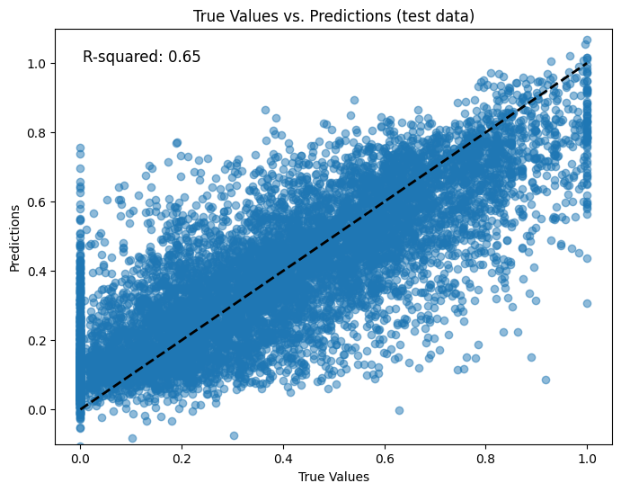
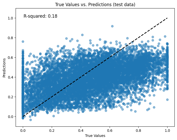
As we can see, the model trained on the regular C3 split performs significantly better on the test set compared to the model trained on the strict C3 split. The \(R^2\) score is much higher and the RMSE is much lower for the regular C3 split. This suggests that although the model generalizes well on predicting binding peptides of seen MHC2 alleles, it struggles to generalize to unseen MHC2 alleles when using the strict C3 split.

Let’s take a look at the prediction plots:

Regular C3 split prediction plot for all MHC2:

Strict C3 split prediction plot for all MHC2:

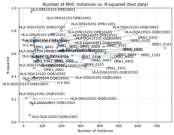
Regular C3 split prediction plot separated by MHC2:

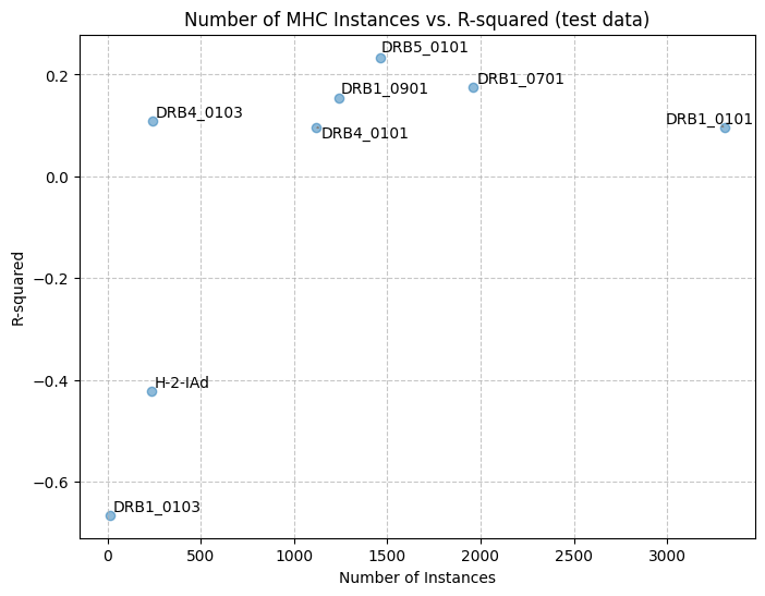
Strict C3 split prediction plot separated by MHC2:

As we can see, while the regular C3 split shows good performance across multiple MHC2 alleles, with some achieving an \(R^2\) score > 0.8, the strict C3 split shows max \(R^2\) score of around 0.2 for the best performing MHC2 allele.

Notably, although the total test sample numbers are the same between the two split, due to the strict nature of the strict C3 split, the variety of MHC2 alleles in the test set is much smaller compared to the regular C3 split. Thus, we are perhaps being a little “strict” in our evaluation, since the strict C3 split has not been evaluated on many MHC2 alleles.

This result suggests important limitations for this model: it predicts well on MHC2 alleles that are present in the training data, but it does not perform well on unseen or novel MHC2 alleles. Perhaps the model is very good at memorizing specific interactions between peptides and MHC2 alleles, but did not learn well the general rules of protein-protein interaction, which is also a significant challenge for many PPI prediction models utilizing pLLMs. Some potential solutions to this issue could include:

• Increasing the diversity of the training data to include a wider range of MHC2 alleles, which may help the model learn more generalizable patterns.
• Incorporating additional features or using more complex model architectures that can capture the underlying biology of peptide binding to MHC2 molecules, rather than relying solely on the embeddings from the pre-trained pLLM.
• Re-train a pLLM on strict data with held out samples, so that the embeddings themselves are less prone to data leakage and more generalizable to unseen data.

Conclusion

In this project, I explored the issue of data leakage in peptide-MHC2 binding prediction models using pre-trained protein language models (pLLMs). I compared two data splitting strategies, a regular C3 split and a strict C3 split, to evaluate the extent of data leakage and its impact on model performance. My findings showed that while the model trained on the regular C3 split performed well on the test set, it struggled to generalize to unseen MHC2 alleles when evaluated using the strict C3 split. This highlights the importance of using stringent data splitting strategies to ensure that models are evaluated on truly unseen data, which is crucial for developing robust and generalizable models in protein binding affinity prediction.

References

• Park, Y., Marcotte, E. Flaws in evaluation schemes for pair-input computational predictions. Nat Methods 9, 1134–1136 (2012).
• Szymborski, Joseph, and Amin Emad. “Data for”A Flaw in Using Pre-trained pLMs in Protein-protein Interaction Inference Models””. bioRxiv, December 5, 2025.
• Lin Z, Akin H, Rao R, Hie B, Zhu Z, Lu W, Smetanin N, Verkuil R, Kabeli O, Shmueli Y, Dos Santos Costa A, Fazel-Zarandi M, Sercu T, Candido S, Rives A. Evolutionary-scale prediction of atomic-level protein structure with a language model. Science. 2023 Mar 17;379(6637):1123-1130. doi: 10.1126/science.ade2574. Epub 2023 Mar 16. PMID: 36927031.