Machine learning for drug sensitivity prediction (Part 2): will deep features improve accuracy?

DepMap

Autoencoder

Multi-omics

Machine Learning

Random Forest

Elastic Net

Caret

Author

Jay Chung

Published

December 8, 2025

In Part 1, I explored using autoencoders (AE) to compress high-dimensional DepMap omics data into deep features. I visualized these features using UMAP and observed that they preserved biological signals related to cell lineage.

In this post (Part 2), I will evaluate whether these deep features actually improve drug sensitivity prediction accuracy compared to using either the full RNA expression data or a feature-selected subset of RNA expression data. The motivation is that deep features may capture complex, non-linear relationships in the data while reducing dimensionality, potentially enhancing model performance. We will focus on two drugs with known biomarkers but with different mechanisms of action: Erlotinib (an EGFR inhibitor) and JQ1 (a BET inhibitor).

Setup and Libraries

library(tidyverse)
library(data.table)
library(ggpubr)
library(caret)
library(doParallel)

Methods: Machine Learning Models

We will use two machine learning algorithms to predict drug sensitivity (log2 fold change) from the DepMap PRISM drug screen data:

Random Forest (RF): A tree-based ensemble method that can capture non-linear relationships.
Elastic Net: A linear regression method with \(l1\) and \(l2\) regularization to prevent overfitting.

We are using the R Caret package for model training and hyperparameter tuning. Caret is a versatile package that provides a unified interface for training various machine learning models with built-in cross-validation and hyperparameter tuning. Documentation can be found here: https://topepo.github.io/caret/.

We will evaluate performance using R-squared (\(R^2\)) on six independent test-train sets across multiple random splits.

Prediction Functions

We define helper functions to perform repeated train-test splits and model training.

# Random Forest Prediction Function
rf_drug_prediction <- function(feature_dat, drug_response, output_file_prefix, n_repeats = 6) {
    r2_values <- c()
    for (i in 1:n_repeats) {
        set.seed(524 + i)
        # 80-20 Train-Test Split
        train_idx <- sample(1:nrow(feature_dat), size = round(0.8 * nrow(feature_dat)), replace = FALSE)
        test_idx <- setdiff(1:nrow(feature_dat), train_idx)

        train_x <- feature_dat[train_idx, ]
        train_y <- drug_response[train_idx]
        test_x <- feature_dat[test_idx, ]
        test_y <- drug_response[test_idx]

        # Train Random Forest with caret
        # caret will perform tuning for all available hyperparameters, and automatically pick the best model (highest R2 on cross-validation)
        set.seed(524 + i)
        rfTune <- train(train_x, train_y,
            method = "rf",
            importance = TRUE,
            ntree = 1000,
            preProcess = c("center", "scale"),
            metric = "Rsquared",
            tuneLength = 10, # tune over 10 different mtry values
            trControl = trainControl(method = "repeatedcv", number = 10, repeats = 3) # 10-fold cross-validation repeated 3 times
        )

        # Predict on Test Set
        rf_pred <- predict(rfTune, newdata = test_x)
        r2 <- cor(rf_pred, test_y, method = "pearson")^2
        r2_values <- c(r2_values, r2)
    }

    # Return R2 values
    return(data.frame(Repeat = 1:n_repeats, R2 = r2_values))
}

# Elastic Net Prediction Function
enet_drug_prediction <- function(feature_dat, drug_response, output_file_prefix, n_repeats = 6) {
    r2_values <- c()
    for (i in 1:n_repeats) {
        set.seed(524 + i)
        # 80-20 Train-Test Split
        train_idx <- sample(1:nrow(feature_dat), size = round(0.8 * nrow(feature_dat)), replace = FALSE)
        test_idx <- setdiff(1:nrow(feature_dat), train_idx)

        train_x <- feature_dat[train_idx, ]
        train_y <- drug_response[train_idx]
        test_x <- feature_dat[test_idx, ]
        test_y <- drug_response[test_idx]

        # Train Elastic Net
        set.seed(524 + i)
        enetTune <- train(train_x, train_y,
            method = "glmnet",
            preProcess = c("center", "scale"),
            metric = "Rsquared",
            tuneLength = 10, # tune over 10 X 10 different alpha/lambda combinations
            # alpha: mixing parameter (0 = ridge, 1 = lasso)
            # lambda: regularization strength
            trControl = trainControl(method = "repeatedcv", number = 10, repeats = 3) # 10-fold cross-validation repeated 3 times
        )

        # Predict on Test Set
        enet_pred <- predict(enetTune, newdata = test_x)
        r2 <- cor(enet_pred, test_y, method = "pearson")^2
        r2_values <- c(r2_values, r2)
    }

    # Return R2 values
    return(data.frame(Repeat = 1:n_repeats, R2 = r2_values))
}

Analysis 1: Erlotinib Prediction

Erlotinib is an EGFR inhibitor used in cancer treatment, which is a type of targeted cancer therapy used primarily to treat certain types of non-small cell lung cancer and pancreatic cancer.

Data Preparation

We load the data and prepare four feature sets:

Full RNA: All high-variance genes.
RNA AE: Deep features from RNA autoencoder.
Multi-omics AE: Deep features from multi-omics autoencoder (including RNA, mutation, and CRISPR).
Selected Top RNA: Top ~4000 gene expressions most correlated with Erlotinib response (a common feature selection strategy).

# Load Data
load("CCLE_24Q2_GE_match_sample_info.RData") # RNA expression in log2(TPM+1)
load("PRISM_24Q2_compound_screen_match_sample_info.RData") # PRISM drug response data in log2 fold change (LFC)
cmpd_dat <- read_csv("Repurposing_Public_24Q2_Extended_Primary_Compound_List.csv") # Compound metadata
load("sample_info_match_biomarkers.RData") # Sample info with DepMap IDs

# ... (Data filtering and matching code similar to Part 1) ...

# Get Erlotinib Response
cmpd_id <- cmpd_dat |>
    filter(Drug.Name == "ERLOTINIB") |>
    pull(IDs)
drug_LFC <- prism_dat_match_sam |> pull(cmpd_id)

Let’s take a look at the PRISM drug screen data. Rows are cell lines and columns are compounds. Values are log2 fold change (LFC) in viability after drug treatment. You can see that there are a lot of NAs here, as many cell lines were not screened with all compounds.

load("PRISM_24Q2_compound_screen_match_sample_info.RData")
prism_dat_match_sam[1:5, 1:5] |> gt::gt()

BRD:BRD-A00047421-001-01-7	BRD:BRD-A00055058-001-01-0	BRD:BRD-A00077618-236-07-6	BRD:BRD-A00092689-236-04-9	BRD:BRD-A00100033-001-08-9
-1.207281	0.5157434	-0.01557664	-0.39512253	-0.4493321
-4.231563	NA	NA	-0.53837559	NA
NA	NA	NA	NA	NA
-3.860672	NA	NA	0.30697134	NA
-2.271411	NA	NA	0.03509603	NA

For brevity, we skip the data cleaning steps here. After filtering for missing data and matching cell lines across datasets, we obtain the final datasets for modeling. We also skip the codes for selecting the top RNA genes correlated with Erlotinib response - it is a simple apply function calculating Pearson correlation for each gene across the transcriptome, and selecting the top genes.

Model Training (Erlotinib)

We train models on all four feature sets.

# Parallel Processing
cl <- makePSOCKcluster(22) # Adjust number of cores as needed
registerDoParallel(cl)

# 1. Full RNA
rf_drug_prediction(ge_dat_final, drug_LFC_final, "full_RNA")
enet_drug_prediction(ge_dat_final, drug_LFC_final, "full_RNA")

# 2. RNA AE Features
rf_drug_prediction(RNA_AE_features_final, drug_LFC_final, "RNA_AE")
enet_drug_prediction(RNA_AE_features_final, drug_LFC_final, "RNA_AE")

# 3. Multi-omics AE Features
rf_drug_prediction(MultiOmics_AE_features_final, drug_LFC_final, "MultiOmics_AE")
enet_drug_prediction(MultiOmics_AE_features_final, drug_LFC_final, "MultiOmics_AE")

# 4. Selected Top RNA
rf_drug_prediction(ge_dat_selected, drug_LFC_final, "selected_top_RNA")
enet_drug_prediction(ge_dat_selected, drug_LFC_final, "selected_top_RNA")

stopCluster(cl)

Results: Erlotinib

Let’s look at the performance (\(R^2\)) of the different models.

# Load results (code omitted for brevity, loading CSVs from results folder)

# Plot Random Forest Results
ggplot(rf_r2_df, aes(x = Model, y = R2, fill = Model, color = Model)) +
    geom_boxplot(alpha = 0.5, outliers = FALSE) +
    geom_jitter(width = 0.2, size = 4) +
    theme_classic(base_size = 20) +
    labs(title = "Random Forest Erlotinib LFC Prediction R2", x = "Model", y = "R2") +
    theme(legend.position = "none")

# Plot Elastic Net Results
ggplot(enet_r2_df, aes(x = Model, y = R2, fill = Model, color = Model)) +
    geom_boxplot(alpha = 0.5, outliers = FALSE) +
    geom_jitter(width = 0.2, size = 4) +
    theme_classic(base_size = 20) +
    labs(title = "Elastic Net Erlotinib LFC Prediction R2", x = "Model", y = "R2") +
    theme(legend.position = "none")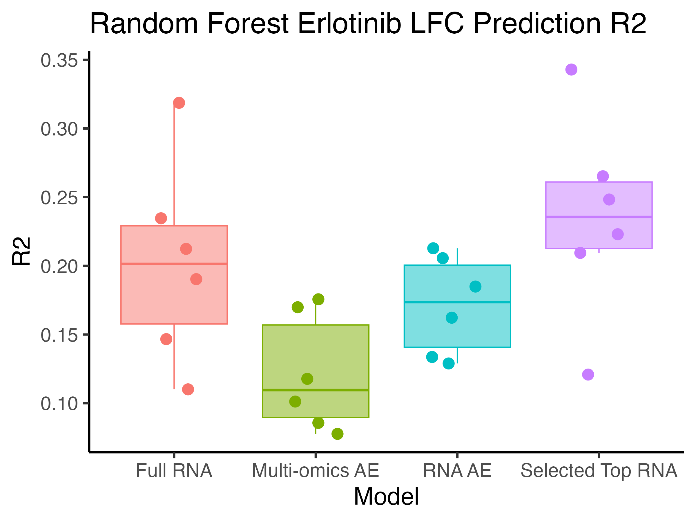

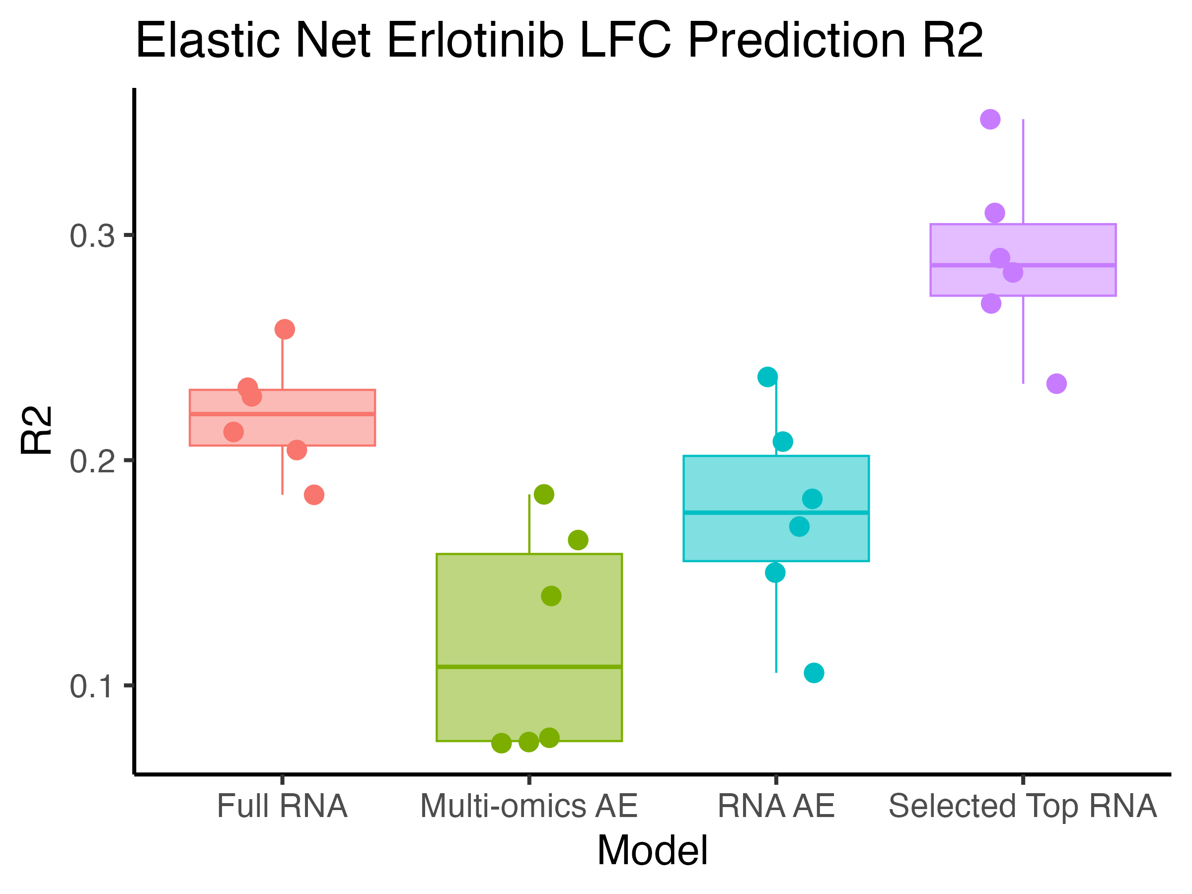
This result is a bit surprising! In both models, the selected top RNA genes outperform all other feature sets. The full RNA set ranks second, while the AE features perform worse. The multi-omics AE features do not seem to add value in this case, and it performs even worse than the RNA AE features alone. I’ll speculate why this might be the case in the summary section. Is this specific to Erlotinib, or a general trend? Let’s check with another drug.

Analysis 2: JQ1 Prediction

Now let’s try to predict sensitivity to JQ1, a BET inhibitor that has a very different mechanism of action compared to Erlotinib.

Model Training (JQ1)

We repeat the same process for JQ1.

Results: JQ1

# ... (Similar plotting code as Erlotinib) ...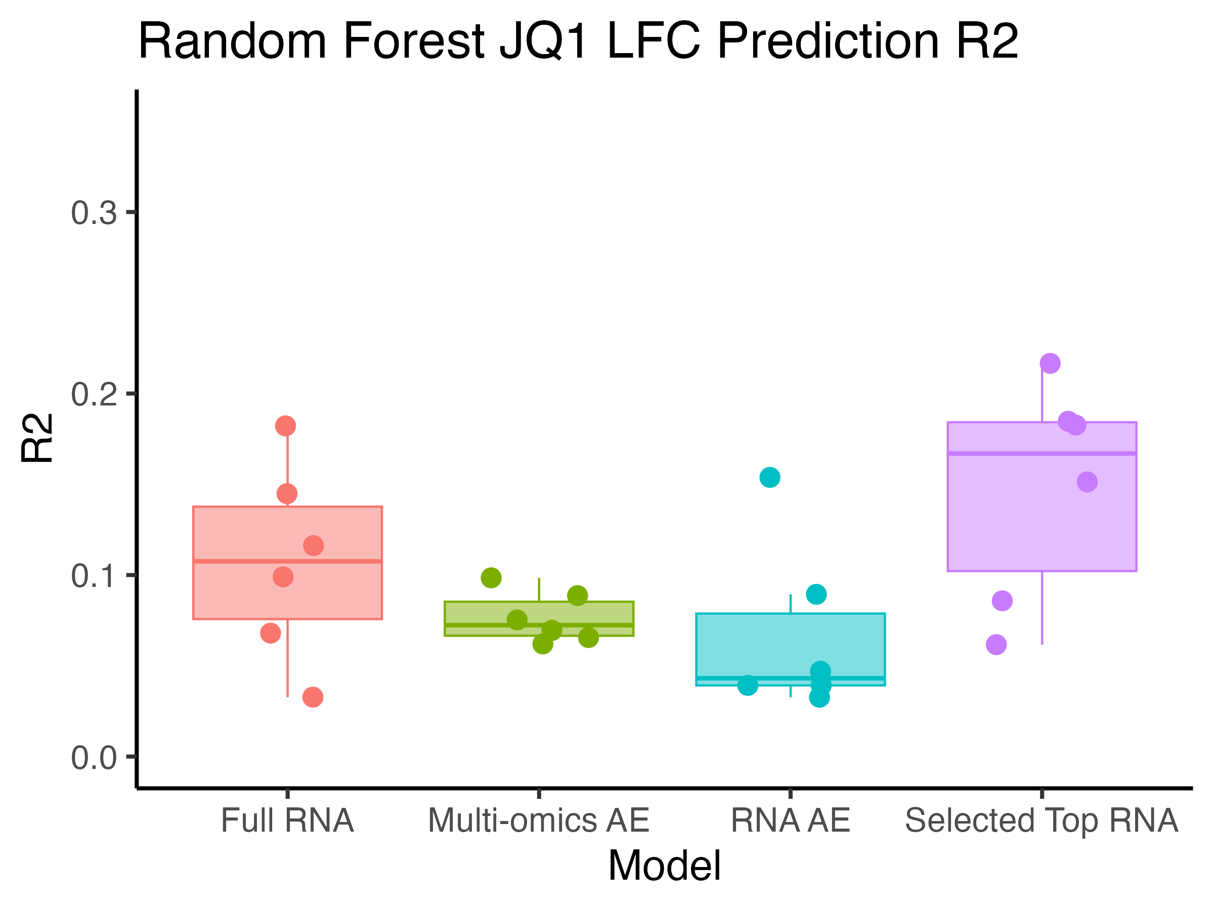

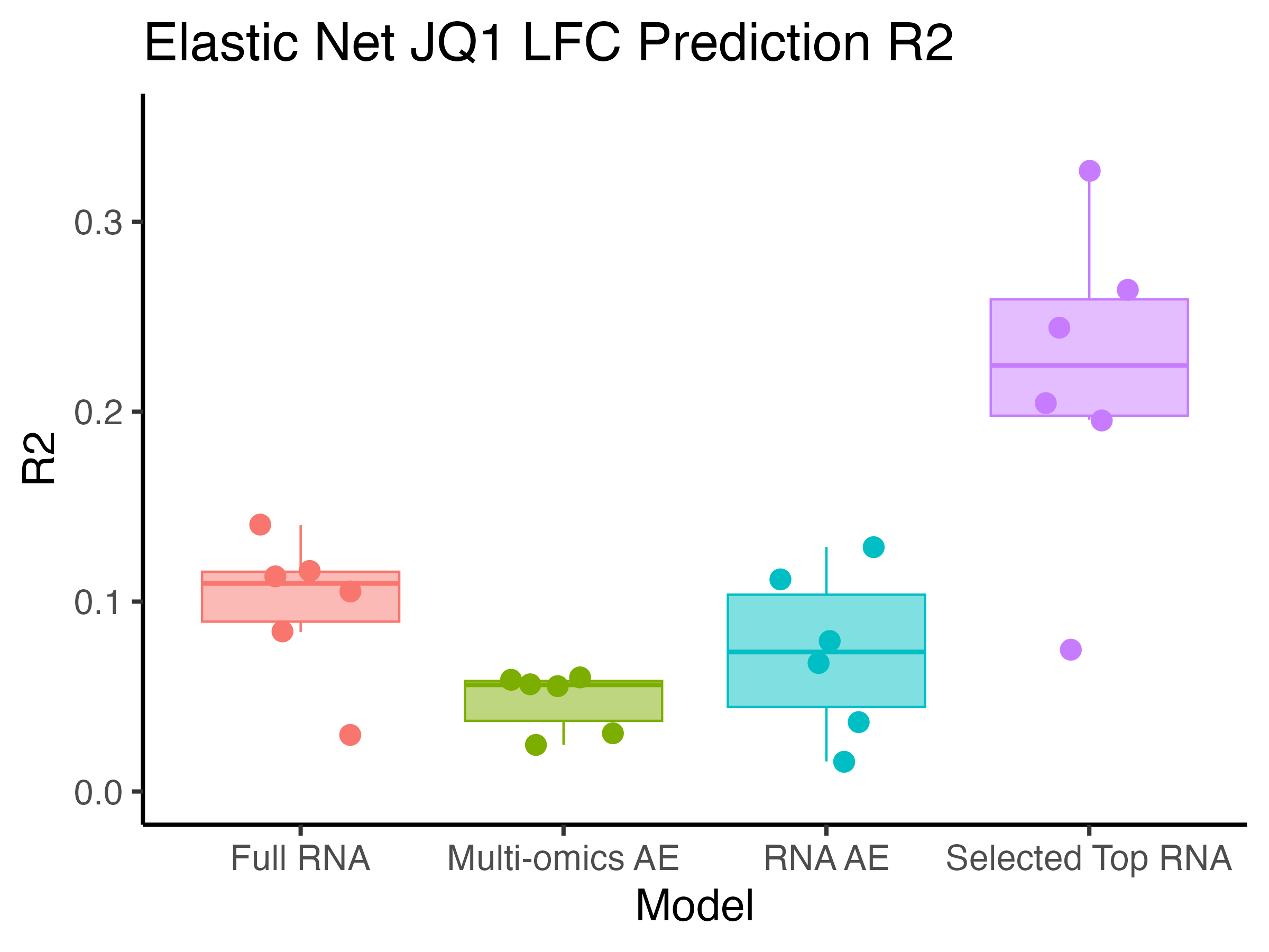
So the conclusion is pretty much the same for JQ1 as well. The selected top RNA genes outperform all other feature sets, followed by the full RNA set. The AE features again perform worse, and adding multi-omics data does not help.

Summary and Conclusions

Contrary to my initial hypothesis, the deep features extracted from autoencoders did not improve drug sensitivity prediction accuracy for either Erlotinib or JQ1. Instead, using a feature-selected subset of RNA expression data yielded the best performance, followed by using the full RNA expression data. The AE features, both RNA-only and multi-omics, underperformed in comparison.

So why is this the case? Here are some possible explanations:

Information Loss: The AE compression may have discarded important predictive information present in the original RNA expression data. Rather than preserving features relevant for drug response, the AE might have prioritized reconstructing general patterns, which in this case is likely the lineage programs between different cell lines. A possible remedy could be to use supervised or semi-supervised autoencoders that incorporate drug response information during training. I also have not experimented with different AE architectures, latent dimensions, or training strategies that might better capture drug response signals.
Multi-omics Integration Challenges: Combining multiple omics data types (RNA, mutation, CRISPR) into a single AE may introduce noise or conflicting signals that obscure relevant features for drug response. Each omics type has different sparsity and scales, making it difficult for a single AE to effectively learn a unified representation. More sophisticated integration methods or separate AEs for each omics type followed by feature fusion might yield better results.
Drug-Specific Biology: Assuming that the AE mainly captures broad biological variation (e.g., lineage), it may not align well with the specific molecular mechanisms driving sensitivity to Erlotinib and JQ1. For example, one of the key biomarkers for Erlotinib sensitivity - EGFR hotspot mutations - are actually quite rare across the cell lines (I’ve counted around 10), and may not be well represented in the AE features. I also did not explore including other omics data types (e.g., proteomics, methylation) that might be relevant for these drugs. Finally, only two drugs were tested here; results may vary for other drugs with different mechanisms of action.
Limitation of ML Models: The Random Forest and Elastic Net models used here may not fully leverage the complex representations learned by the AEs. More advanced models (e.g., deep neural networks) that can capture non-linear relationships in the AE feature space might yield different results. However, one significant drawback of deep learning is that it generally requires much larger training datasets to avoid overfitting, which may not be feasible with the limited number of cell lines available in a regular drug screen.

Interestingly, between the 2 models, the Elastic Net seemed to slightly outperform Random Forest in most cases. Given that the training time for Elastic Net is significantly shorter than Random Forest, this suggests that for these specific drug response predictions, simpler linear models with regularization may be more effective than more complex non-linear models.

So there you have it! In the next and final part of this series, I will revisit the concept I introduced in my first post: enhancing statistical power of drug biomarker detection by ML. I will use the best performed model (selected top RNA with Elastic Net) to expand drug prediction to all DepMap available cell lines (e.g., there are only ~500 cell lines screened for Erlotinib, but DepMap has close to 2000 cell lines), and see if we can better recover known sensitivity biomarkers.

References

DepMap Portal: https://depmap.org/portal/
Caret Package Documentation: https://topepo.github.io/caret/
Applied Predictive Modeling by Kuhn and Johnson: https://www.springer.com/gp/book/9781461468486
An Introduction to Statistical Learning by James et al.: https://www.statlearning.com/